Technical indicators are great and effective, but all of them never fail to have one specific drawback — the false trading signals, and trading influenced by them might lead to catastrophic results. To tackle this problem, it is best to introduce two different technical indicators, whose characteristics vary from one another, to the trading strategy, and by doing so, we could filter the false trading signals from the authentic ones.

In this article, we will try building a trading strategy with two technical indicators which are Bollinger Bands, and Stochastic Oscillator in Python. We will also backtest the strategy and compare the returns with those of the SPY ETF (an ETF designed specifically to track the movement of the S&P 500 market index). Without further ado, let’s dive into the article!

Quick jump:

1 Bollinger Bands
2 Stochastic Oscillator
3 Trading strategy
4 Implementation in Python
5 Final Thoughts!

Bollinger Bands

Before jumping on to explore Bollinger Bands, it is essential to know what Simple Moving Average (SMA) is. Simple Moving Average is the average price of a stock given a specified period of time. Now, Bollinger Bands are trend lines plotted above and below the SMA of the given stock at a specific standard deviation level. To understand Bollinger Bands better, have a look at the following chart that represents the Bollinger Bands of the Apple stock calculated with SMA 20.

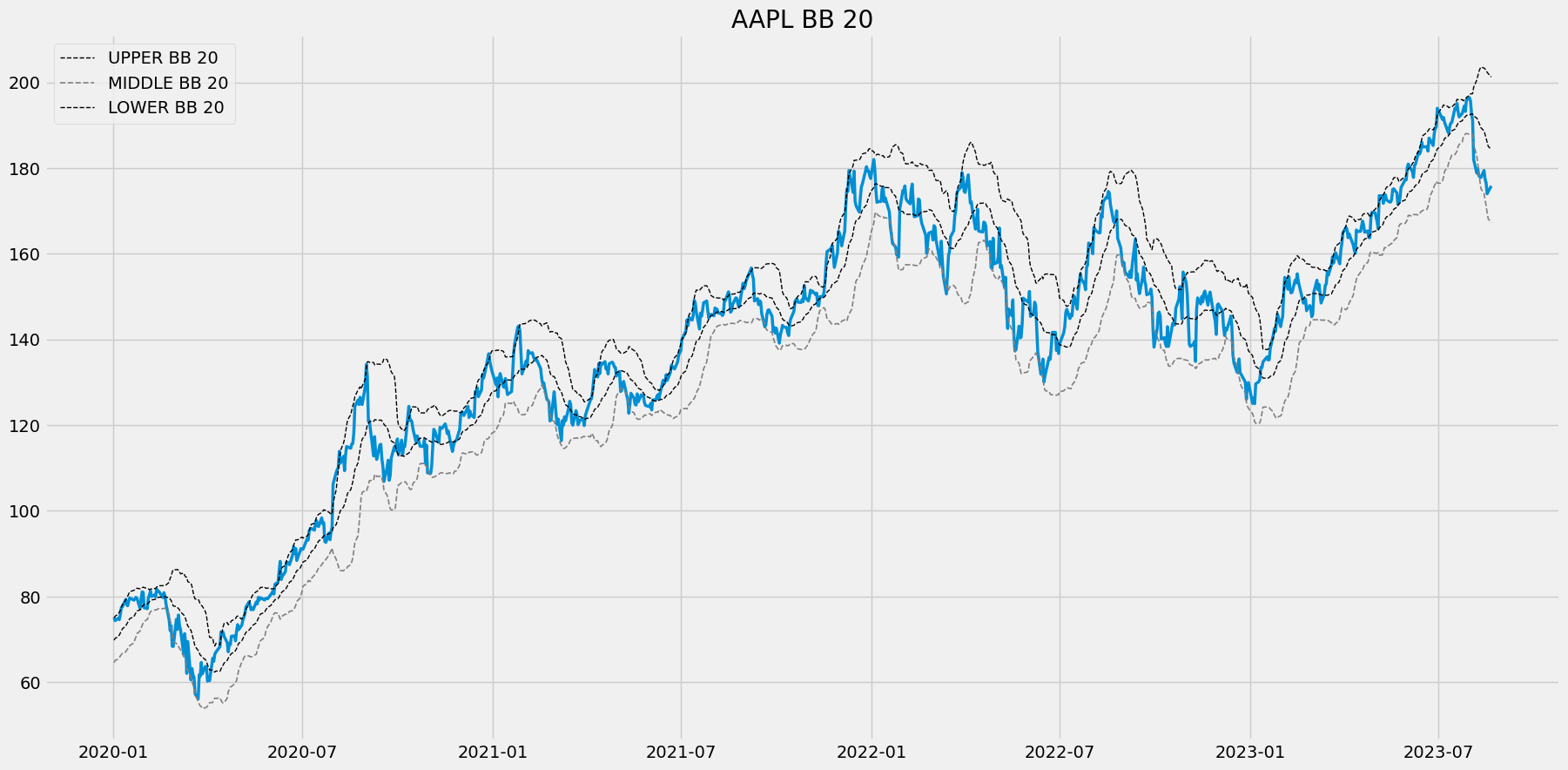
Bollinger Bands are great to observe the volatility of a given stock over a period of time. The volatility of a stock is observed to be lower when the space or distance between the upper and lower band is less. Similarly, when the space or distance between the upper and lower band is more, the stock has a higher level of volatility. While observing the chart, you can observe a trend line named ‘MIDDLE BB 20’ which is SMA 20 of the Apple stock. The formula to calculate both upper and lowers bands of stock are as follows:

UPPER_BB = STOCK SMA + SMA STANDARD DEVIATION * 2
LOWER_BB = STOCK SMA - SMA STANDARD DEVIATION * 2

Stochastic Oscillator

Stochastic Oscillator is a momentum-based leading indicator that is widely used to identify whether the market is in the state of overbought or oversold. This leads to our next question. What is overbought and oversold in a concerning market? A stock is said to be overbought when the market’s trend seems to be extremely bullish and bound to consolidate. Similarly, a stock reaches an oversold region when the market’s trend seems to be extremely bearish and has the tendency to bounce.

The values of the Stochastic Oscillator always lie between 0 to 100 due to its normalization function. The general overbought and oversold levels are considered as 70 and 30 respectively, but it could vary somewhat. The Stochastic Oscillator comprises two main components:

%K Line: This line is the most important and core component of the Stochastic Oscillator indicator. It is otherwise known as the Fast Stochastic indicator. The sole purpose of this line is to express the current state of the market (overbought or oversold). This line is calculated by subtracting the lowest price the stock has reached over a specified number of periods from the closing price of the stock and this difference is then divided by the value calculated by subtracting the lowest price the stock has reached over a specified number of periods from the highest stock price. The final value is arrived at by multiplying the value calculated from the above-mentioned steps by 100. The way to calculate the %K line with the most popular setting of 14 as the number of periods can be represented as follows:

%K = 100 * ((14 DAY CLOSING PRICE - 14 DAY LOWEST PRICE) - (14 DAY HIGHEST PRICE - 14 DAY LOWEST PRICE))

%D Line: Otherwise known as the Slow Stochastic Indicator, it is the moving average of the %K line for a specified period. It is also known as the smooth version of the %K line as the line graph of the %D line will look smoother than the %K line. The standard setting of the %D line is 3 as the number of periods.

That’s the whole process of calculating the components of the Stochastic Oscillator. Now, let’s analyze a chart where Apple’s closing price data is plotted along with its Stochastic Oscillator calculated with 14 and 3 as the lookback periods of the %K line and % D line respectively to build a solid understanding of the indicator and how it’s being used.

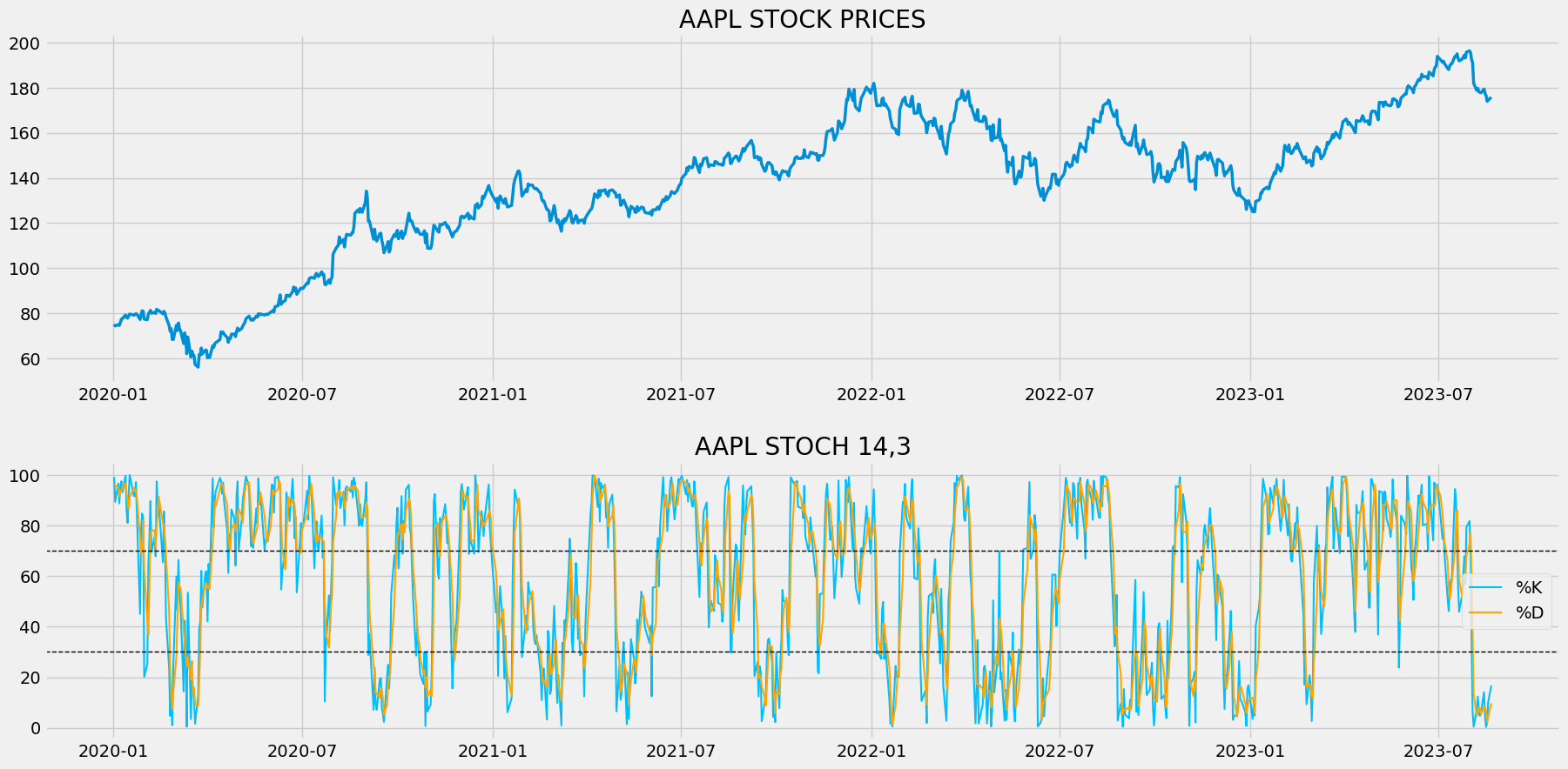
The plot is subdivided into two panels: The upper panel and the lower panel. The upper panel represents the line plot of the closing price of Apple. The lower panel comprises the components of the Stochastic Oscillator. Being a leading indicator, the stochastic oscillator cannot be plotted alongside the closing price as the values of the indicator and the closing price vary a lot. So, it is plotted apart from the closing price (below the closing price in our case).

The components %K line and %D line we discussed before are plotted in blue and orange respectively. You can also notice two additional black dotted lines above and below the %K and %D line. It is an additional component of the Stochastic Oscillator known as Bands. These bands are used to highlight the region of overbought and oversold. If both the %K and %D line crosses above the upper band, then the stock is considered to be overbought. Likewise, when both the %K and %D line crosses below the lower band, the stock is considered to be oversold.

Trading strategy

Now that we have built some basic understanding of what both the technical indicators are all about. Let’s proceed to the trading strategy we are going to implement in this article using Bollinger Bands and the Stochastic Oscillator.

Our trading strategy will reveal a buy signal if the previous day readings of the components of the Stochastic Oscillator are above 30, current-day components’ readings are below 30, and the last closing price is below the lower band. Similarly, a sell signal is revealed whenever the Stochastic Oscillator’s components’ readings are below 70, current components’ readings are above 70, and the last closing price is above the upper band. The strategy can be represented as follows:

IF PREV_ST_COM > 30 AND CUR_ST_COMP < 30 AND CL < LOWER_BB ==> BUY
IF PREV_ST_COM > 70 AND CUR_ST_COMP < 70 AND CL < UPPER_BB ==> SELL

where,

PRE_ST_COM = Previous Day Stochastic Oscillator components' readings
CUR_ST_COM = Current Day Stochastic Oscillator components' readings
CL = Last Closing Price
LOWER_BB = Current Day Lower Band reading
UPPER_BB = Current Day Upper Band reading

That’s it! This concludes our theory part and let’s move on to the programming part where we will use Python to first build the indicators from scratch, construct the discussed trading strategy, backtest the strategy on Apple stock data, and finally compare the results with that of SPY ETF. Let’s do some coding! Before moving on, a note on disclaimer: This article’s sole purpose is to educate people, and it must be considered as an information piece but not as investment advice.

Implementation in Python

The coding part is classified into various steps as follows:

1. Importing Packages
2. Extracting Stock Data from EODHD
3. Bollinger Bands Calculation
4. Stochastic Oscillator Calculation
5. Creating the Trading Strategy
6. Creating our Position
7. Backtesting
8. SPY ETF Comparison

We will be following the order mentioned in the above list and buckle up your seat belts to follow every upcoming coding part.

Step-1: Importing Packages

Importing the required packages into the Python environment is a non-skippable step. The primary packages are going to be Pandas to work with data, NumPy to work with arrays and for complex functions, Matplotlib for plotting purposes, and Requests to make API calls. The secondary packages are going to be Math for mathematical functions and Termcolor for font customization (optional).

Python Implementation:

# IMPORTING PACKAGES

import pandas as pd
import requests
import numpy as np
import matplotlib.pyplot as plt
from math import floor
from termcolor import colored as cl

plt.rcParams[‘figure.figsize’] = (20, 10)
plt.style.use(‘fivethirtyeight’)

With the required packages imported into Python, we can proceed to fetch historical data for Apple using EODHD’s OHLC split-adjusted data API endpoint.

Step-2: Extracting Stock Data from EODHD

In this phase, we’re set to retrieve the historical stock data for Apple using the OHLC split-adjusted API endpoint provided by EODHD. It’s important to note that EOD Historical Data (EODHD)is a reliable provider of financial APIs, encompassing an extensive array of market data, including historical data and economic news. Be sure to possess an EODHD account and access your secret API key, a crucial element for data extraction via the API.

Python Implementation:

# EXTRACTING STOCK DATA

def get_historical_data(symbol, start_date):
    api_key = 'YOUR API KEY'
    api_url = f'https://eodhistoricaldata.com/api/technical/{symbol}?order=a&fmt=json&from={start_date}&function=splitadjusted&api_token={api_key}'
    raw_df = requests.get(api_url).json()
    df = pd.DataFrame(raw_df)
    df.date = pd.to_datetime(df.date)
    df = df.set_index('date')
    return df

aapl = get_historical_data('AAPL', '2010-01-01')
aapl.tail()

Output:

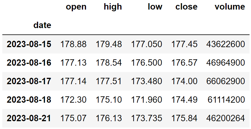
Code Explanation: We begin by defining a function named ‘get_historical_data,’ which takes the stock symbol (‘symbol’) and the start date for historical data (‘start_date’) as parameters. Inside the function, we define the API key and URL, then retrieve the historical data in JSON format using the ‘get’ function and store it in the ‘raw_df’ variable. After cleaning and formatting the raw JSON data, we return it as a Pandas dataframe. Finally, we call this function to fetch Apple’s historical data from the start of 2010 and store it in the ‘aapl’ variable.

Step-3: Bollinger Bands calculation

In this step, we are going to calculate the components of the Bollinger Bands by following the methods and formula we discussed before.

Python Implementation:

# BOLLINGER BANDS CALCULATION

def sma(data, lookback):
    sma = data.rolling(lookback).mean()
    return sma

def get_bb(data, lookback):
    std = data.rolling(lookback).std()
    upper_bb = sma(data, lookback) + std * 2
    lower_bb = sma(data, lookback) - std * 2
    middle_bb = sma(data, lookback)
    return upper_bb, lower_bb, middle_bb

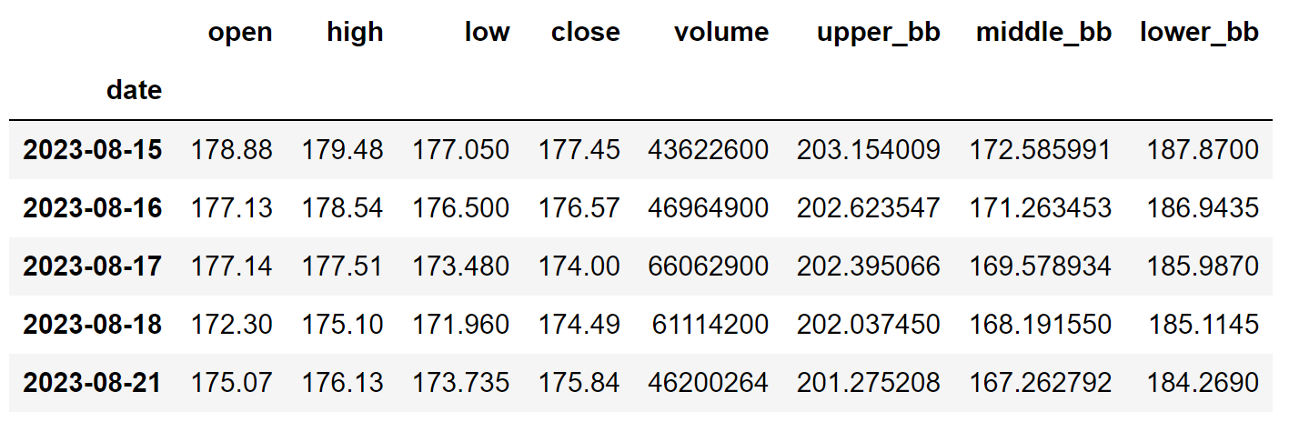
aapl['upper_bb'], aapl['middle_bb'], aapl['lower_bb'] = get_bb(aapl['close'], 20)
aapl = aapl.dropna()
aapl.tail()

Output:

Code Explanation: The above can be classified into two parts: SMA calculation, and the Bollinger Bands calculation.

SMA calculation: Firstly, we are defining a function named ‘sma’ that takes the stock prices (‘data’), and the number of periods (‘lookback’) as the parameters. Inside the function, we are using the ‘rolling’ function provided by the Pandas package to calculate the SMA for the given number of periods. Finally, we are storing the calculated values into the ‘sma’ variable and return them.

Bollinger Bands calculation: We are first defining a function named ‘get_bb’ that takes the stock prices (‘data’), and the number of periods as parameters (‘lookback’). Inside the function, we are using the ‘rolling’ and the ‘std’ function to calculate the standard deviation of the given stock data and stored the calculated standard deviation values into the ‘std’ variable. Next, we are calculating Bollinger Bands values using their respective formulas, and finally, we are returning the calculated values. We are storing the Bollinger Bands values into our ‘aapl’ dataframe using the created ‘bb’ function.

Step-4: Stochastic Oscillator calculation

In this step, we are going to calculate the components of the Stochastic Oscillator by following the methods and formula we discussed before.

Python Implementation:

# STOCHASTIC OSCILLATOR CALCULATION

def get_stoch_osc(high, low, close, k_lookback, d_lookback):
    lowest_low = low.rolling(k_lookback).min()
    highest_high = high.rolling(k_lookback).max()
    k_line = ((close - lowest_low) / (highest_high - lowest_low)) * 100
    d_line = k_line.rolling(d_lookback).mean()
    return k_line, d_line

aapl['%k'], aapl['%d'] = get_stoch_osc(aapl['high'], aapl['low'], aapl['close'], 14, 3)
aapl.tail()

Output:

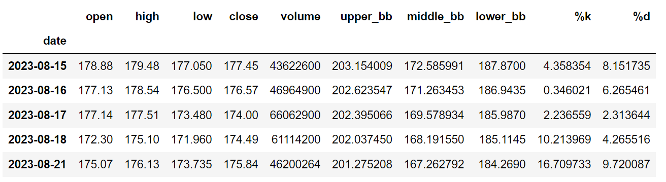
Code Explanation: We are first defining a function named ‘get_stoch_osc’ that takes a stock’s high (‘high’), low (‘low’), closing price data (‘close’), and the lookback periods of the %K line (‘k_lookback’) and the %D line (‘d_lookback’) respectively as parameters. Inside the function, we are first calculating the lowest low and highest high data points for a specified number of periods using the ‘rolling’, ‘min’, and ‘max’ functions provided by the Pandas packages and stored the values into the ‘lowest_low’, and ‘highest_high’ variables.

Then comes the %K line calculation where we are substituting the formula into our code and stored the readings into the ‘k_line’ variable, followed by that, we are calculating the %D line which is simply taking the SMA of the %K line readings for a specified number of periods. Finally, we are returning the values and calling the function to store Apple’s Stochastic Oscillator readings with 14 and 3 as the lookback periods of the %K and %D line respectively.

Step-5: Creating the trading strategy

In this step, we are going to implement the discussed Bollinger Bands and Stochastic Oscillator trading strategy in Python.

Python Implementation:

# TRADING STRATEGY

def bb_stoch_strategy(prices, k, d, upper_bb, lower_bb):
    buy_price = []
    sell_price = []
    bb_stoch_signal = []
    signal = 0
    
    for i in range(len(prices)):
        if k[i-1] > 30 and d[i-1] > 30 and k[i] < 30 and d[i] < 30 and prices[i] < lower_bb[i]:
            if signal != 1:
                buy_price.append(prices[i])
                sell_price.append(np.nan)
                signal = 1
                bb_stoch_signal.append(signal)
            else:
                buy_price.append(np.nan)
                sell_price.append(np.nan)
                bb_stoch_signal.append(0)
        elif k[i-1] < 70 and d[i-1] < 70 and k[i] > 70 and d[i] > 70 and prices[i] > upper_bb[i]:
            if signal != -1:
                buy_price.append(np.nan)
                sell_price.append(prices[i])
                signal = -1
                bb_stoch_signal.append(signal)
            else:
                buy_price.append(np.nan)
                sell_price.append(np.nan)
                bb_stoch_signal.append(0)
        else:
            buy_price.append(np.nan)
            sell_price.append(np.nan)
            bb_stoch_signal.append(0)
    
    sell_price[-1] = prices[-1]
    bb_stoch_signal[-1] = -1
    return buy_price, sell_price, bb_stoch_signal

buy_price, sell_price, bb_stoch_signal = bb_stoch_strategy(aapl['close'], aapl['%k'], aapl['%d'], aapl['upper_bb'], aapl['lower_bb'])

Code Explanation: First, we are defining a function named ‘bb_stoch_strategy’ which takes the stock prices (‘prices’), %K line readings (‘k’), %D line readings (‘d’), Upper Bollinger band (‘upper_bb’), and the Lower Bollinger band (‘lower_bb’) as parameters.

Inside the function, we are creating three empty lists (buy_price, sell_price, and bb_stoch_signal) in which the values will be appended while creating the trading strategy.

After that, we are implementing the trading strategy through a for-loop. Inside the for-loop, we are passing certain conditions, and if the conditions are satisfied, the respective values will be appended to the empty lists. If the condition to buy the stock gets satisfied, the buying price will be appended to the ‘buy_price’ list, and the signal value will be appended as 1 representing to buy the stock. Similarly, if the condition to sell the stock gets satisfied, the selling price will be appended to the ‘sell_price’ list, and the signal value will be appended as -1 representing to sell the stock. Finally, we are returning the lists appended with values. Then, we are calling the created function and store the values into their respective variables.

Step-6: Creating our Position

In this step, we are going to create a list that indicates 1 if we hold the stock or 0 if we don’t own or hold the stock.

Python Implementation:

# POSITION

position = []
for i in range(len(bb_stoch_signal)):
    if bb_stoch_signal[i] > 1:
        position.append(0)
    else:
        position.append(1)
        
for i in range(len(aapl['close'])):
    if bb_stoch_signal[i] == 1:
        position[i] = 1
    elif bb_stoch_signal[i] == -1:
        position[i] = 0
    else:
        position[i] = position[i-1]
        
k = aapl['%k']
d = aapl['%d']
upper_bb = aapl['upper_bb'] 
lower_bb = aapl['lower_bb']
close_price = aapl['close']
bb_stoch_signal = pd.DataFrame(bb_stoch_signal).rename(columns = {0:'bb_stoch_signal'}).set_index(aapl.index)
position = pd.DataFrame(position).rename(columns = {0:'bb_stoch_position'}).set_index(aapl.index)

frames = [close_price, k, d, upper_bb, lower_bb, bb_stoch_signal, position]
strategy = pd.concat(frames, join = 'inner', axis = 1)

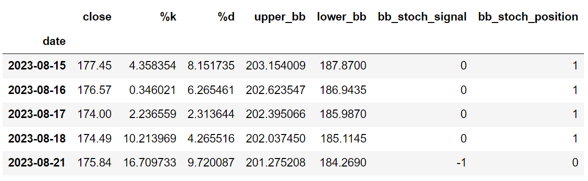
strategy.tail()

Output:

Code Explanation: First, we are creating an empty list named ‘position’. We are passing two for-loops, one is to generate values for the ‘position’ list to just match the length of the ‘signal’ list. The other for-loop is the one we are using to generate actual position values.

Inside the second for-loop, we are iterating over the values of the ‘signal’ list, and the values of the ‘position’ list get appended concerning which condition gets satisfied. The value of the position remains 1 if we hold the stock or remains 0 if we sold or don’t own the stock. Finally, we are doing some data manipulations to combine all the created lists into one dataframe.

From the output being shown, we can see that in the first four rows, our position in the stock has remained 1 (since there isn’t any change in the trading signal) but our position suddenly turned to 0 as we sold the stock when the trading signal represents a buy signal (-1). Our position will remain -1 until some changes in the trading signal occur. Now it’s time to implement some backtesting processes!

Step-7: Backtesting

Before moving on, it is essential to know what backtesting is. Backtesting is the process of seeing how well our trading strategy has performed on the given stock data. In our case, we are going to implement a backtesting process for our Bollinger Bands Stochastic Oscillator trading strategy over the Apple stock data.

Python Implementation:

# BACKTESTING

aapl_ret = pd.DataFrame(np.diff(aapl['close'])).rename(columns = {0:'returns'})
bb_stoch_strategy_ret = []

for i in range(len(aapl_ret)):
    returns = aapl_ret['returns'][i]*strategy['bb_stoch_position'][i]
    bb_stoch_strategy_ret.append(returns)
    
bb_stoch_strategy_ret_df = pd.DataFrame(bb_stoch_strategy_ret).rename(columns = {0:'bb_stoch_returns'})
investment_value = 100000
bb_stoch_investment_ret = []

for i in range(len(bb_stoch_strategy_ret_df['bb_stoch_returns'])):
    number_of_stocks = floor(investment_value/aapl['close'][i])
    returns = number_of_stocks*bb_stoch_strategy_ret_df['bb_stoch_returns'][i]
    bb_stoch_investment_ret.append(returns)

bb_stoch_investment_ret_df = pd.DataFrame(bb_stoch_investment_ret).rename(columns = {0:'investment_returns'})
total_investment_ret = round(sum(bb_stoch_investment_ret_df['investment_returns']), 2)
profit_percentage = floor((total_investment_ret/investment_value)*100)
print(cl('Profit gained from the BB STOCH strategy by investing $100k in AAPL : {}'.format(total_investment_ret), attrs = ['bold']))
print(cl('Profit percentage of the BB STOCH strategy : {}%'.format(profit_percentage), attrs = ['bold']))

Output:

Profit gained from the BB STOCH strategy by investing $100k in AAPL : 315318.91
Profit percentage of the BB STOCH strategy : 315%

Code Explanation: First, we are calculating the returns of the Apple stock using the ‘diff’ function provided by the NumPy package and we have stored it as a dataframe in the ‘aapl_ret’ variable. Next, we are passing a for-loop to iterate over the values of the ‘aapl_ret’ variable to calculate the returns we gained from our trading strategy, and these returns values are appended to the ‘bb_stoch_strategy_ret’ list. Next, we are converting the ‘bb_stoch_strategy_ret’ list into a dataframe and storing it in the ‘bb_stoch_strategy_ret_df’ variable.

Next comes the backtesting process. We are going to backtest our strategy by investing a hundred thousand USD into our trading strategy. So first, we are storing the amount of investment into the ‘investment_value’ variable. After that, we are calculating the number of Apple stocks we can buy using the investment amount. You can notice that I’ve used the ‘floor’ function provided by the Math package because, while dividing the investment amount by the closing price of Apple stock, it spits out an output with decimal numbers. The number of stocks should be an integer but not a decimal number. Using the ‘floor’ function, we can cut out the decimals. Remember that the ‘floor’ function is way more complex than the ‘round’ function. Then, we are passing a for-loop to find the investment returns followed by some data manipulation tasks.

Finally, we are printing the total return we got by investing a hundred thousand into our trading strategy and it is revealed that we have made an approximate profit of $315,000 in around thirteen-and-a-half years with a profit percentage of 315%. That’s great! Now, let’s compare our returns with SPY ETF (an ETF designed to track the S&P 500 stock market index) returns.

Step-8: SPY ETF Comparison

While this step is optional, it is highly recommended as it enables us to assess the performance of our trading strategy against a benchmark (SPY ETF). Here, we’ll extract SPY ETF data using the ‘get_historical_data’ function and compare the returns from the SPY ETF with the returns generated by our trading strategy applied to Apple stock.

Python Implementation:

def get_benchmark(start_date, investment_value):
    spy = get_historical_data('SPY', start_date)['close']
    benchmark = pd.DataFrame(np.diff(spy)).rename(columns = {0:'benchmark_returns'})
    
    investment_value = investment_value
    benchmark_investment_ret = []
    
    for i in range(len(benchmark['benchmark_returns'])):
        number_of_stocks = floor(investment_value/spy[i])
        returns = number_of_stocks*benchmark['benchmark_returns'][i]
        benchmark_investment_ret.append(returns)

    benchmark_investment_ret_df = pd.DataFrame(benchmark_investment_ret).rename(columns = {0:'investment_returns'})
    return benchmark_investment_ret_df

benchmark = get_benchmark('2010-01-01', 100000)

investment_value = 100000
total_benchmark_investment_ret = round(sum(benchmark['investment_returns']), 2)
benchmark_profit_percentage = floor((total_benchmark_investment_ret/investment_value)*100)
print(cl('Benchmark profit by investing $100k : {}'.format(total_benchmark_investment_ret), attrs = ['bold']))
print(cl('Benchmark Profit percentage : {}%'.format(benchmark_profit_percentage), attrs = ['bold']))
print(cl('BB STOCH Strategy profit is {}% higher than the Benchmark Profit'.format(profit_percentage - benchmark_profit_percentage), attrs = ['bold']))

Output:

Benchmark profit by investing $100k : 156261.12
Benchmark Profit percentage : 156%
BB STOCH Strategy profit is 159% higher than the Benchmark Profit

Code Explanation: The code used in this step is almost similar to the one used in the previous backtesting step but, instead of investing in Apple, we are investing in SPY ETF by not implementing any trading strategies. From the output, we can see that our Bollinger Bands Stochastic Oscillator trading strategy has outperformed the SPY ETF by 159%. That’s awesome!

Final Thoughts!

After an exhaustive process of crushing both theory and programming parts, we have successfully built a trading strategy with two technical indicators which actually make some good returns.

In my opinion, considering two technical indicators to build a trading strategy is the most fundamental and important step in technical analysis and we have to make sure that we do it the right way. This will help us from overcoming one of the huge obstacles while using technical indicators which are false signals and that’s great because making our trades align with non-authentic signals would lead to bizarre results and ultimately leads to depleting the capital as a whole.

Talking about improvements, one way to improve this article and take it to the next level would be to create a trading strategy that is realistic in nature. In this article, our program would buy the stocks if the corresponding condition gets satisfied and the same for selling the stock but when implemented in the real-world market, the scenario would be different.

For example, for each trade being made in the real-world market, some fraction of the capital would be transferred to the broker as commission, but in our strategy, we did not consider factors like this and even has some impact on our returns. So, constructing our trading strategy in realistic ways might help us get more practical insights.

With that being said, you’ve reached the end of the article. Hope you learned something new and useful from this article.

Bollinger Bands

Stochastic Oscillator

Trading strategy

Implementation in Python

Step-1: Importing Packages

Step-2: Extracting Stock Data from EODHD

Step-3: Bollinger Bands calculation

Step-4: Stochastic Oscillator calculation

Step-5: Creating the trading strategy

Step-6: Creating our Position

Step-7: Backtesting

Step-8: SPY ETF Comparison

Final Thoughts!

Related Articles

Backtesting Technical Analysis Strategies with Excel(SMA, RSI, MACD)

Portfolio Risk Management with Excel

Microsoft Excel Stock Market Dashboard

Real-Time Market Data in Google Sheets with WebSocket

Portfolio Risk Analytics using Google Sheets

Using Delisted Stocks for Backtesting a 3-EMA Strategy with Python