

The Discounted Cash Flow (DCF) model stands as one of the most widely employed financial models for investment evaluation. This model plays a crucial role in estimating the intrinsic value of a public company’s stock. The intrinsic share price is determined through an analysis of the company’s current and anticipated future cash flows.
In essence, the intrinsic value reflects the perceived worth of a company’s stock based on its fundamental financials. Comparing this intrinsic value with the current market valuation of a company provides valuable insights into the investment potential. This comparison aids in gauging whether a particular firm is a sound investment by indicating if its stock is currently undervalued or overvalued.
Quick jump:
A real case-study: Tesla
For this case study, we will employ the EODHD Python Library to seamlessly download financial statement data directly into our Jupyter notebook via the API service. In our illustrative example, we focus our analysis on Tesla stock (ticker = “TSLA.US”), a subject that sparks considerable debate on Wall Street due to its intriguing valuation. Our analysis kicks off by retrieving the most recent company data using the client.get_fundamental_equity function. This function can be used to obtain the three main documents that constitute an annual company report: the Balance Sheet, Income Statement, and Cash Flow Statement. Collectively, these documents offer a comprehensive overview of the company’s financial health and performance, forming the cornerstone of our analytical process.
import eod
client = EodHistoricalData(api_key)1. Use the “demo” API key to test our data from a limited set of tickers without registering: AAPL.US | TSLA.US | VTI.US | AMZN.US | BTC-USD | EUR-USD
Real-Time Data and all of the APIs (except Bulk) are included without API calls limitations with these tickers and the demo key.
2. Register to get your free API key (limited to 20 API calls per day) with access to: End-Of-Day Historical Data with only the past year for any ticker, and the List of tickers per Exchange.
3. To unlock your API key, we recommend to choose the subscription plan which covers your needs.
stock_ticker = "TSLA.US"
#download BS, IS, CFS from EOD historical data
BalanceSheet = client.get_fundamental_equity(stock_ticker, filter_='Financials::Balance_Sheet::yearly')
IncomeStat = client.get_fundamental_equity(stock_ticker, filter_='Financials::Income_Statement::yearly')
CashFlowStat = client.get_fundamental_equity(stock_ticker, filter_='Financials::Cash_Flow::yearly')
OutShares = client.get_fundamental_equity(stock_ticker, filter_='SharesStats::SharesOutstanding')
# transpose and concatenate
df_bal = pd.DataFrame(BalanceSheet).T
df_inc = pd.DataFrame(IncomeStat).T
df_cfs = pd.DataFrame(CashFlowStat).T
df_all = pd.concat([df_bal, df_inc, df_cfs], axis=1).sort_index()
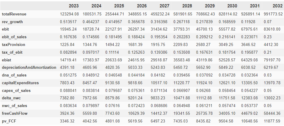
df_all = df_all.loc[:, ~df_all.columns.duplicated()] #remove duplicated columnsWe begin by executing some preprocessing steps to present our data in a more suitable format. This involves tasks such as converting data to float type and replacing datetime entries with the corresponding year. Given the large size of the table, we filter it taking a few sample columns and show the result below:
#convert all None values to np.NaN datatypes
df = df_all.iloc[-10 :, 3:,].applymap(lambda x: float(x) if x is not None else np.NaN)
df.index = pd.to_datetime(df.index)
df.index = df.index.year
df = df.applymap(format_value)
df.head(10)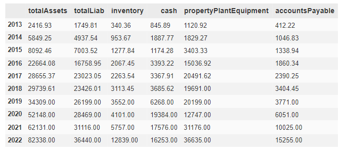
The table serves as a snapshot for the entire dataframe, offering a glimpse into its structure ensuring that the content is displayed accurately. To facilitate visualization, the values have been converted to floating-point numbers and are expressed in millions of dollars ($).
Preparing the DCF ingredients
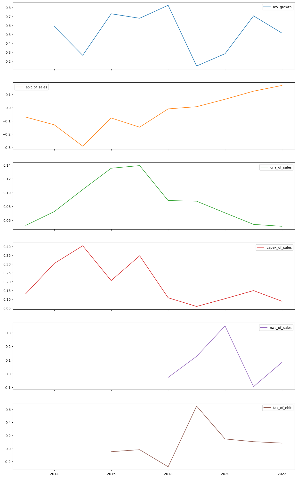
After retrieving the financial company data, we can now compute the value of all the variables required in a Discounted Cash Flow model:
- % Revenue Growth
- % Ebit/Sales
- % D&A/Sales
- % Capex/Sales
- % Δ Net Working Capital/ Sales
- % Tax/Ebit
- Ebiat = Earning before interests after taxes
# compute % of sales and % of ebit variables
df["rev_growth"] = df["totalRevenue"].pct_change()
df["delta_nwc"] = df["netWorkingCapital"].diff()
df["ebit_of_sales"] = df["ebit"]/df["totalRevenue"]
df["dna_of_sales"] = df["depreciationAndAmortization"]/df["totalRevenue"]
df["capex_of_sales"] = df["capitalExpenditures"]/df["totalRevenue"]
df["nwc_of_sales"] = df["delta_nwc"]/df["totalRevenue"]
df["tax_of_ebit"] = df["taxProvision"]/df["ebit"]
df["ebiat"] = df["ebit"] - df["taxProvision"]
last_year = df.iloc[-1, :]
Also, we store data from the most recent financial statement in the variable last_year. This will be helpful to calculate our projections through linear interpolation.
Assumptions
The assumptions in a Discounted Cash Flow (DCF) analysis are foundational elements that significantly influence the accuracy and reliability of the valuation. The DCF method relies on projecting future cash flows and discounting them back to their present value. Assumptions about growth rates, discount rates, terminal values, and other factors shape these projections. An example of how the sensitivity to changes in these assumptions impact the final valuation will be shown in the last chapter.
In this case study, we develop a 10-year DCF, implying that our projections extend until the year 2032. The other variables are assumed as follows:
- N = years of projections = 10
- % Revenue Growth = 7%
- % Ebit/Sales = 23%
- % D&A/Sales = 3%
- % Capex/Sales = 5%
- % Δ Net Working Capital/ Sales = 5%
- % Tax/Ebit = 21%
- TGR = 2.5%
n = 10
revenue_growth_T = 0.07
ebit_perc_T = 0.23
tax_perc_T = 0.21
dna_perc_T = 0.03
capex_perc_T = 0.05
nwc_perc_T = 0.05
TGR = 0.025
Creating the DCF projections
Now that our model components are in place, it is opportune to delve into considerations regarding the company’s future values. In this scenario, the goal is to model the trajectories of the variables in accordance with our expectations of the company and the industry future developments. For the sake of simplicity, we make the assumption of a linear trend for values from time t+1 to T. Thus we assume a constant rate of change of our model variables. Despite being a stringent assumption, linear interpolation is often use to model the value at intermediate dates between the starting value and the last projection.
def interpolate(initial_value, terminal_value, nyears):
    return np.linspace(initial_value, terminal_value, nyears)
years = range(df.index[-1]+1, df.index[-1] + n + 1)
df_proj = pd.DataFrame(index=years, columns=df.columns)
# linear interpolation
df_proj["rev_growth"] = interpolate(last_year["rev_growth"], revenue_growth_T, n)
df_proj["ebit_of_sales"] = interpolate(last_year["ebit_of_sales"], ebit_perc_T, n)
df_proj["dna_of_sales"] = interpolate(last_year["dna_of_sales"], dna_perc_T, n)
df_proj["capex_of_sales"] = interpolate(last_year["capex_of_sales"], capex_perc_T, n)
df_proj["tax_of_ebit"] = interpolate(last_year["tax_of_ebit"], tax_perc_T, n)
df_proj["nwc_of_sales"] = interpolate(last_year["nwc_of_sales"], nwc_perc_T, n)
# cumulative values
df_proj["totalRevenue"] = last_year["totalRevenue"] *(1+df_proj["rev_growth"]).cumprod()
df_proj["ebit"] = last_year["ebit"] *(1+df_proj["ebit_of_sales"]).cumprod()
df_proj["capitalExpenditures"] = last_year["capitalExpenditures"] *(1+df_proj["capex_of_sales"]).cumprod()
df_proj["depreciationAndAmortization"] = last_year["depreciationAndAmortization"] *(1+df_proj["dna_of_sales"]).cumprod()
df_proj["delta_nwc"] = last_year["delta_nwc"] *(1+df_proj["nwc_of_sales"]).cumprod()
df_proj["taxProvision"] = last_year["taxProvision"] *(1+df_proj["tax_of_ebit"]).cumprod()
df_proj["ebiat"] = df_proj["ebit"] - df_proj["taxProvision"]The last step before moving to the WACC estimation is to calculate the FCF by using the equation below:

df_proj["freeCashFlow"] = df_proj["ebiat"] + df_proj["depreciationAndAmortization"] - df_proj["capitalExpenditures"] - df_proj["delta_nwc"]Weighted Average Cost of Capital (WACC)
For the calculation of the WACC, we will need to retrieve more data from the EOD database:
- Company’s Beta
- Company’s Market Capitalization
- 10-year US Treasury Rate, as proxy for the risk-free rate
- Yield-to-Maturity of Tesla’s bonds
- Equity Risk Premium, from Damodaran website
Cost of Equity
According to the Capital Asset Pricing Model (CAPM), the cost of equity is often calculated as the expected rate of return on the company’s equity, and it is represented by the formula

Thus, we first need to collect data on the company’s market capitalization and beta i.e. the sensitivity to market returns, the risk-free rate (here we use 10-y US treasury as proxy) and the equity risk premium
# company's beta and marketcap
beta = client.get_fundamental_equity(stock_ticker, filter_='Technicals::Beta')
marketcap = client.get_fundamental_equity(stock_ticker, filter_='Highlights::MarketCapitalization')

# risk-free rate
US10Y = client.get_prices_eod("US10Y.INDX", period='d', order='a')
US10Y = pd.DataFrame(US10Y).set_index("date")["adjusted_close"]
US10Y.rename("10Y", inplace=True)
rf_rate = US10Y.values[-1] /100

# get ERP
excel_url = "https://www.stern.nyu.edu/~adamodar/pc/datasets/histimpl.xls"
df_ERP = pd.read_excel(excel_url, skiprows=6)
df_ERP = df_ERP.dropna(subset=["Year"]).iloc[:-1, :].set_index("Year")
ERP = df_ERP["Implied ERP (FCFE)"].values[-1]
CostOfEquity = beta*(ERP) + rf_rateTesla Inc.’s cost of equity stands at 17.9%. This is attributed, on one hand, to the stock’s heightened sensitivity to market returns (beta), and on the other hand, to the elevated interest rate environment recorded in 2023.
Cost of Debt
We will use the yield-to-maturity (YTM) of bond issues as proxy for the Tesla’s cost of debt. Bond data can be retrieved either through the Search API or Exchange API function. In the latter case, we will need to pass the code BOND as exchange name.
import requests
url = f'https://eodhd.com/api/exchange-symbol-list/BOND?api_token={apikey}&fmt=json&delisted=1'
data = requests.get(url).json()
bond_issues = pd.DataFrame(data)
tsla_bond_issues = bond_issues[bond_issues["Name"].str.contains("Tesla")]
YTM = np.zeros(len(tsla_bond_issues))
today = datetime.now()
c = 0
for i in tsla_bond_issues["Code"]:
bond_data = client.get_fundamentals_bonds(i, bond_only=1)
YTM[c] = bond_data["YieldToMaturity"]
c+=1
tsla_bond_issues["YTM"] = YTM
CostOfDebt = tsla_bond_issues["YTM"].mean() /100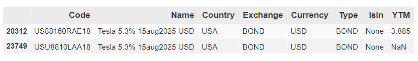
Hence, we will adopt 3.885% as a proxy for the company’s cost of debt. The final step involves applying the Weighted Average Cost of Capital (WACC) formula. This is a weighted average, with the weights representing the debt and equity portions in the company’s balance sheet. The resulting equation provides us with the discount rate, which will be applied to project and anticipate future cash flow projections.

where C(D) and C(E) are the cost of debt and cost of equity, respectively, and T is the tax rate.
Assets =  last_year["totalAssets"]
Debt = last_year["totalLiab"]
total = marketcap + Debt
AfterTaxCostOfDebt = CostOfDebt * (1-tax_perc_T)
WACC = (AfterTaxCostOfDebt*Debt/total) + (CostOfEquity*marketcap/total)
In this example, we calculate a WACC of 17.2% for Tesla, a figure that stands notably higher than market standards. This elevated value can be attributed to the positive equity market performance, elevated interest rates, and Tesla’s heightened sensitivity to equity market returns.
Calculating present value of FCF
After estimating the company’s projections and WACC, it’s time to calculate the present value of the FCF using the WACC as the discount rate:

def calculate_present_value(cash_flows, discount_rate):
    # Calculate the present value using: PV = CF / (1 + r)^t + TV/(1 + r)^T
    present_values_cf = [cf / (1 + discount_rate) ** t for t, cf in enumerate(cash_flows, start=1)]
    return present_values_cf
df_proj["pv_FCF"] = calculate_present_value(df_proj["freeCashFlow"].values, WACC)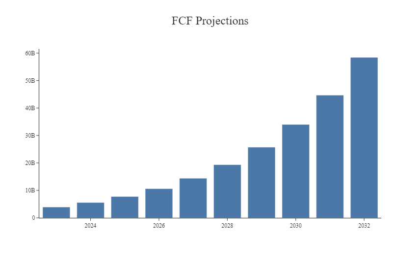
Finally we compute the Terminal Value i.e. the present value of all future cash flows beyond the explicit forecast period; in our case, 2032. The formula for the Terminal Value is:
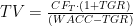
where TGR is the Terminal Growth Rate and represents the rate at which we expect the free cash flows of Tesla to grow beyond the explicit forecast period.
TV = df_proj["freeCashFlow"].values[-1] *(1+TGR) / (WACC - TGR)
pv_TV = TV/(1+WACC)**n
As a final step, we sum up the present value of FCF and the terminal value to obtain the Enterprise Value. From here, we can derive the Equity Value by subtracting the outstanding debt and adding cash. The implied Share Price is finally obtained by dividing the Equity Value by the number of outstanding shares.
Ent_Value = np.sum(df_proj["pv_FCF"]) + pv_TV
Cash = last_year["cash"]
Eq_Value = Ent_Value - Debt + Cash
ImpliedSharePrice = Eq_Value/OutShares
Based on our assumptions, we obtained a Tesla share price of 42$ per shares which is very low considering that it is currently trading at 250$. This results is due to the very high cost of equity (17.9%) and extremely low level of company’s debt. As showed in the next chapter, for more moderate levels of WACC ~8% we can easily obtain valuation above 300$. Investors are invited to use assumption values in line with their own expectations and views of the market.
Sensitivity analysis
In the context of DCF modelling, a sensitivity analysis is a technique used to understand how changes in certain key variables impact the calculated net present value (NPV) of a project or investment, and consequently, the implied share price. In this example, we vary the WACC and TGR to observe the impact of these variables on the final valuation. Intuitively, a higher WACC significantly reduces the future value of FCF and, consequently, the company’s valuation. Conversely, the TGR works in the opposite way, positively influencing the terminal value (TV) and thereby enhancing the overall valuation.
waccs = np.linspace(0.06, 0.18, 25)
tgrs = np.linspace(0.01, 0.04, 25)

# Create a meshgrid for cost of debt and growth rate
waccs_mesh, tgrs_mesh = np.meshgrid(waccs, tgrs)

# Calculate NPV for each combination of cost of debt and growth rate
dcf_results = np.zeros_like(waccs_mesh)
for i in range(len(tgrs)):
    for j in range(len(waccs)):
         dcf_results[i, j] = Discount_Cash_Flow(df,  n=10, OutShares=OutShares, revenue_growth_T = 0.07, ebit_perc_T = 0.23,  tax_perc_T = 0.21, dna_perc_T = 0.03, capex_perc_T = 0.05, nwc_perc_T = 0.05, WACC = waccs[j],  TGR = tgrs[i])

fig = plt.figure()
ax = fig.add_subplot(111, projection='3d')
ax.plot_surface(waccs_mesh, tgrs_mesh, dcf_results, cmap='viridis')

ax.set_xlabel('WACC')
ax.set_ylabel('TGR')
ax.set_zlabel('Implied Share Price')
ax.set_title('Tesla Sensitivity Analysis')

plt.show()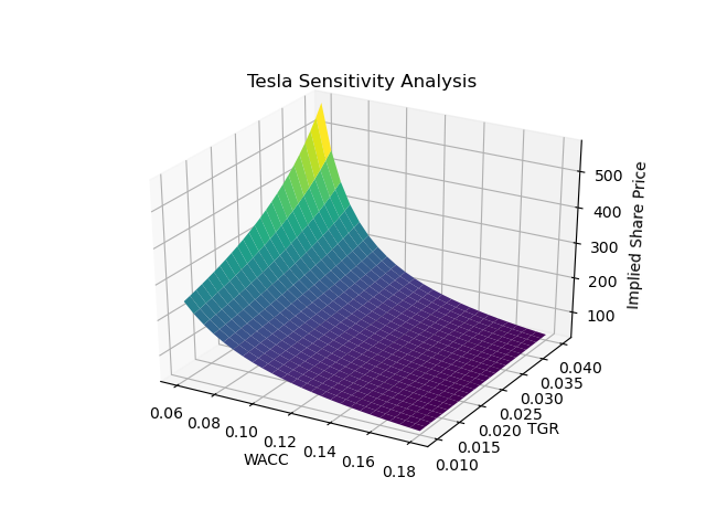
This analytical approach allows for a more comprehensive assessment of the model’s robustness and provides insights into the sensitivity of the valuation to fluctuations in key parameters.
Conclusion
In conclusion, this tutorial has provided a comprehensive guide on how to perform a Discounted Cash Flow (DCF) analysis in Python, empowering users to assess the intrinsic value of a company’s stock based on its future cash flows. By leveraging the EODHD Pyhton Financial Library, we could download all key financial information in an efficient way and cover all the key steps to get the implicit share price, including data preprocessing, assumption setting, and the actual DCF calculation.
Our journey also delved into the fundamental concept of Free Cash Flow (FCF), providing a detailed formula and explanation of its significance in the DCF calculation. This metric serves as the cornerstone for estimating a company’s intrinsic value by accounting for its operational efficiency, capital expenditures, and overall financial health. Finally, we showed a practical approach to effectively compute the Weighted Average Cost of Capital (WACC) based on the initial data.
Full code available here
Website: baglinifinance.com