

Using Python Pandas to backtest algorithmic trading strategies
There are so many trading strategies and candlestick patterns out there, but the question is — how do you measure the performance? This is where a financial data APIs like the one by EODHD are really helpful. You can simulate how a strategy or candlestick pattern would perform using historical data. I wanted to develop a backtesting tool using the data science Pandas library for Python. I’ve created a proof of concept for it, and it’s working well. I will talk you through the thought process I went through while creating it.
Quick jump:
What will we need?
- The EODHD official Python library.
- Trading data converted into a Pandas dataframe (date, open, high, close, low, volume)
- Configurable test settings (balance_base, account_balance, buy_order_quote)
- Apply our buy and sell signals in some form to our data (set_buy_signals, set_sell_signals)
- We will need to be able to iterate through our data (in this case our Pandas dataframe)
- Log the outcome of each completed order
Building up the code
To start off I’m going to create a “pandas-bt.py” file and import the “eodhd” library. You may or may not already have the “eodhd” library installed. I would recommend reinstalling it anyway, which will carry out an upgrade to the latest version if necessary.
% python3 -m pip install eodhd -UThe starter code will look like this:
# pandas-bt.py

import sys
import pandas as pd
from eodhd import APIClient


def get_ohlc_data() -> pd.DataFrame:
    """Return a DataFrame of OHLC data"""

    api = APIClient("<Your_API_Key>")
    df = api.get_historical_data(symbol="HSPX.LSE", interval="d", iso8601_start="2020-01-01", iso8601_end="2023-09-08")
    df.drop(columns=["symbol", "interval", "close"], inplace=True)
    df.rename(columns={"adjusted_close": "close"}, inplace=True)
    print(df)

    return pd.DataFrame([], columns=["date", "open", "high", "low", "close"])


def main() -> int:
    """Backtest a strategy using pandas"""

    df = get_ohlc_data()
    print(df)

    return 0


if __name__ == '__main__':
    sys.exit(main())
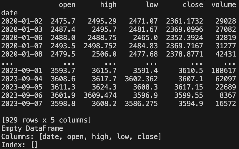
929 days of S&P 500 data should be enough.
Trading strategy
This will work with any trading strategy or candlestick pattern. All we need to do is add a new feature called “buy_signal” with a 1 on a buy signal otherwise a 0. We will do the same for “sell_signal“.
For the purposes of this demonstration I’m going to use a EMA12/EMA26 crossover strategy.
def get_ohlc_data() -> pd.DataFrame:
    """Return a DataFrame of OHLC data"""

    api = APIClient("<Your_API_Key>")
    df = api.get_historical_data(symbol="HSPX.LSE", interval="d", iso8601_start="2020-01-01", iso8601_end="2023-09-08")
    df.drop(columns=["symbol", "interval", "close"], inplace=True)
    df.rename(columns={"adjusted_close": "close"}, inplace=True)

    return df


def main() -> int:
    """Backtest a strategy using pandas"""

    df = get_ohlc_data()

    df["ema12"] = df["close"].ewm(span=12, adjust=False).mean()
    df["ema26"] = df["close"].ewm(span=26, adjust=False).mean()

    df["ema12gtema26"] = df["ema12"] > df["ema26"]
    df["buy_signal"] = df["ema12gtema26"].ne(df["ema12gtema26"].shift())
    df.loc[df["ema12gtema26"] == False, "buy_signal"] = False  # noqa: E712
    df["buy_signal"] = df["buy_signal"].astype(int)

    df["ema12ltema26"] = df["ema12"] < df["ema26"]
    df["sell_signal"] = df["ema12ltema26"].ne(df["ema12ltema26"].shift())
    df.loc[df["ema12ltema26"] == False, "sell_signal"] = False  # noqa: E712
    df["sell_signal"] = df["sell_signal"].astype(int)

    df.drop(columns=["ema12", "ema26", "ema12gtema26", "ema12ltema26"], inplace=True)

    print(df)
    return 0
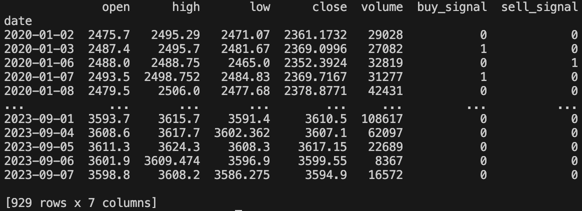
What we have now is an OHLC dataset for the S&P 500 daily with the “buy_signal” set to 1 when the EMA12 crosses above the EMA26, and a “sell_signal” when the EMA12 crosses below the EMA26.
Backtesting the strategy
We now want to iterate through the dataset and simulate orders.
Add this code instead of the “print(df)” line, above the “return 0“.
    balance_base = 0
    account_balance = 1000
    buy_order_quote = 1000
    is_order_open = False
    orders = []
    sell_value = 0

    for index, row in df.iterrows():
        if row["buy_signal"] and is_order_open == 0:
            is_order_open = 1

            if sell_value < 1000 and sell_value > 0:
                buy_order_quote = sell_value
            else:
                buy_order_quote = 1000

            buy_amount = buy_order_quote / row["close"]
            balance_base += buy_amount
            account_balance += sell_value

            order = {
                "timestamp": index,
                "account_balance": account_balance,
                "buy_order_quote": buy_order_quote,
                "buy_order_base": buy_amount
            }

            account_balance -= buy_order_quote

        if row["sell_signal"] and is_order_open == 1:
            is_order_open = 0

            sell_value = buy_amount * row["close"]
            balance_base -= buy_amount

            order["sell_order_quote"] = sell_value
            order["profit"] = order["sell_order_quote"] - order["buy_order_quote"]
            order["margin"] = (order["profit"] / order["buy_order_quote"]) * 100

            orders.append(order)
        print(index)

    df_orders = pd.DataFrame(orders)
    print(df_orders)
“balance_base” is the quantity of the stock we have at the beginning of the simulation, which in this case is 0.
“account_balance” is the quote currency we are starting with for the simulation, in this case £1000.
“buy_order_quote” is the requested size of the order, in this case £1000. If the account balance is less than £1000, then the order will be whatever is available.
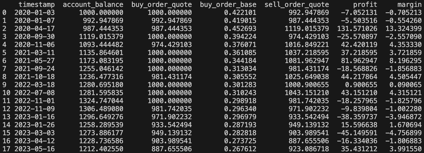
This analysis shows that if we traded every EMA12/EMA26 crossover from January 3rd, 2020, until September 16th, 2023, we would start with £1000 and have £1212.40 at the end, resulting in a 21.24% return over 2.75 years. While this performance isn’t extraordinary, it’s reasonable.
Please note this doesn’t factor in exchange fees. For more accurate results, consider applying applicable fees. The point is, you can apply any strategy and see how it would perform over the same period. Once you have a winning formula, give it a go!