
In this article, we explore the application of the Generalized Autoregressive Conditional Heteroskedasticity (GARCH) model. It’s used to capture volatility clustering in time series, particularly to analyze NVIDIA stock returns. Volatility, often seen as the heartbeat of financial markets, is crucial. It’s a key component to incorporate in any forecasting model for better predictions. We start by exploring the fundamentals of the GARCH model. We’ll unravel its components and underlying principles. Then, we follow a step-by-step implementation. This ranges from data retrieval to result interpretation. The goal is to provide a thorough understanding of GARCH implementation. The aim is to capture the dynamic nature of volatility in financial time series data.
Data
To retrieve our data through the EODHD API, we first need to download and import the EOD Python package. Then, authenticate using your personal API key. It’s recommendable to save your API keys in the environment variable. We are going to use the Historical Data API, which is available in our plans. However, some plans have limited time depth (1-30 years).
pip install eodimport os
# load the key from the environment variables
api_key = os.environ['API_EOD']
import eod
client = EodHistoricalData(api_key)1. Use the “demo” API key to test our data from a limited set of tickers without registering:
AAPL.US | TSLA.US | VTI.US | AMZN.US | BTC-USD | EUR-USD
Real-Time Data and all of the APIs (except Bulk) are included without API calls limitations with these tickers and the demo key.
2. Register to get your free API key (limited to 20 API calls per day) with access to:
End-Of-Day Historical Data with only the past year for any ticker, and the List of tickers per Exchange.
3. To unlock your API key, we recommend choosing the subscription plan which covers your needs.
GARCH Model Basics
Tim Bollerslev developed the Generalized Autoregressive Conditional Heteroskedasticity (GARCH) model in 1986. It was designed to address financial time series exhibiting heteroskedasticity. Heteroskedasticity refers to variance changes over time. The GARCH(p, q) model extends the Autoregressive Conditional Heteroskedasticity (ARCH) model introduced by Robert Engle in 1982.
The equation governing the conditional variance (


Here’s a quick guide to the components:
is the constant term.
and
are coefficients.
represents the squared residuals from previous time periods.
The GARCH model posits that the conditional variance at any given time is a function. It depends on past squared observations and past conditional variances.
To understand the fluctuations in market volatility, researchers estimate GARCH model parameters using a method called maximum likelihood estimation (MLE). This approach entails finding the parameters that best fit the model to the observed market data, based on a specific probability distribution, typically assuming that the market returns follow a normal distribution. Once accurately estimated, these parameters render the GARCH model a highly effective tool for predicting future market volatility. This aids market participants in better preparing for potential changes in risk, thereby enhancing their decision-making processes.
Application
Step 1 – Check for ARMA structure
The choice between directly applying GARCH or first testing for an ARMA model depends on the specific characteristics of your data and the objectives of your analysis. In some cases, it may still be beneficial to test for an ARMA model before fitting a GARCH model, especially if there are clear patterns in the mean of the series that need to be captured. To better understand the process and the example presented below, refer to my previous article.
Step 2 – Testing for ARCH effect
Depending on the necessity of implementation of an ARMA model on the time series, one can either access the residuals of the ARMA regression model or deal directly with the data, and of course, the latter needs to be stationary. In the first case, one should square the residuals to assess the presence of conditional heteroskedasticity, which refers to the time-varying volatility in a time series. In the second case, simply square the data.
To proceed with the test, utilize the Autocorrelation and Partial Autocorrelation functions as seen here. It is important to notice that unlike the test for Autoregressive and Moving Average identification, the orders of p and q are reversed. Meaning p will be identified in the ACF and q in the PACF. This method is not the most robust test to identify ARCH effects, but it is a useful tool to identify the lag order for each term. Important to notice that in financial data, a p and q of order one will do the trick [GARCH(1,1)].
ARCH-LM Test
A more robust approach to identifying ARCH effects is the ARCH-LM test which can be used in Python with the code below.
from arch import arch_model

model = arch_model(data2)  #Squared residuals from ARMA or data squared
result = model.fit()
arch_test = result.arch_lm_test(lags = 12)
print(arch_test)
To better understand the properties and results of the ARCH-LM test, we will apply it in a real-life example.
Step 3 – Model GARCH
Upon the identification of ARCH effects and its lag orders, the following step would be to implement it into a model. To do so, simply identify the mean as zero, constant (allowing it to be estimated from the data), or autoregressive in the case of the residual of an AR process. Then, input the orders of p and q to obtain a Generalized Autoregressive Conditional Heteroskedasticity model.
Step 4 – Analyze results
The last step of implementing GARCH is to access the residuals from the regression to identify is the model was able to capture all the information on the time series and a white noise was obtained. In this process, the same procedure in step 2 is applied. If the residuals are a white noise the ACF and PACF should have no significant lags. A useful tool to formally test the absence of autocorrelation is the Ljung-Box test, which will be implemented and explained in our example and can be accessed through the function below.
def Ljung(series):
    result_df = acorr_ljungbox(series, lags=list(range(1, 21)), return_df=True)
    print(result_df)
GARCH Example: NVIDIA Stock
This analysis is a continuation from the previous example given on the ARIMA Analysis on Stock Returns article.
To retrieve data, we utilize the Official EOD Python API library. Our process begins with gathering data for NVIDIA dating back to March 2014. Information on stocks is accessible through the use of the get_historical_data function.
start = "2014-03-01"

prices = api.get_historical_data("NVDA", interval="d", iso8601_start=start,
                              iso8601_end="2024-03-01")["adjusted_close"].astype(float)
prices.name = "NVDA"

returns = np.log(prices[1:].values) - np.log(prices[0:-1].values)
Analyzing Residuals
After obtaining our AR(1) model, we proceed to test for ARCH effects on the squared residuals from the regression. An important reminder to check for p in the ACF and q in the PACF, unlike the identification done in ARMA. When estimated on financial data, ARCH models usually involve large number of p of significant lags, this why the Generalized component of the model is important.
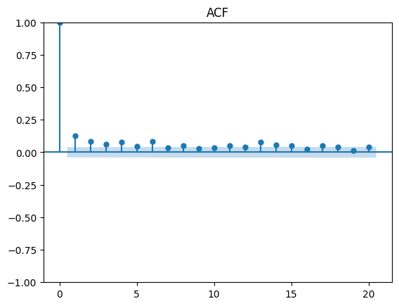
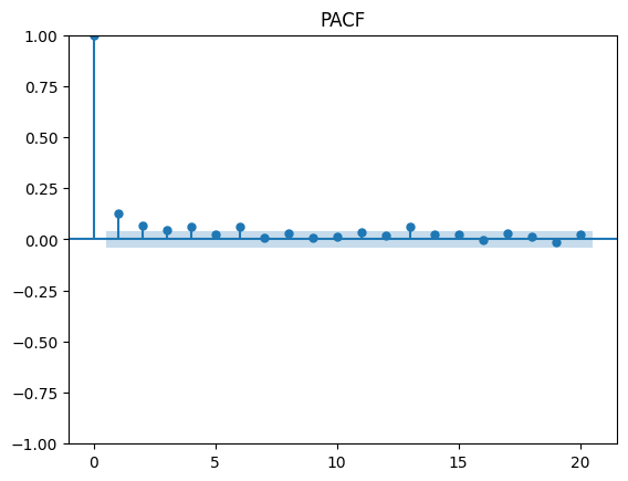
As seen above, both the ACF and PACF have a geometric decay and seem to have relevant significance up to lag 4 and 3 respectively. Since we are dealing with financial returns, usually a GARCH(1,1) gives a good fit (parsimonious model).
ARCH-LM Test
To implement a more robust test, we can utilize the code provided previously on the squared residuals to obtain the following output:
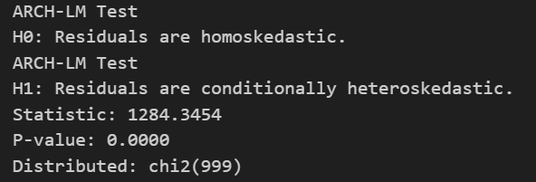
The null hypothesis is that the residuals are homoscedastic, meaning they have constant variance. The alternative hypothesis is that the residuals present volatility clustering, meaning they are heteroscedastic.
With a p-value of 0 we reject the null hypothesis for any given significance level on the one-tailed Chi-squared distribution. Therefore, the residuals contain ARCH effects as perceived on the ACF and PACF.
AR(1)-GARCH(1,1) Model
To build a model out of our observations we shall use the following code:
ARCH_model = arch_model(returns, mean = 'AR', lags = 1, vol='Garch', p=1, q=1)
result = ARCH_model.fit()
print(result.summary())

result.plot()
plt.show()
Notice this time we input our actual returns, and we are no longer using residuals squared as the goal is to model our observations and not to test our dataset. Upon running the regression, the following results were obtained:
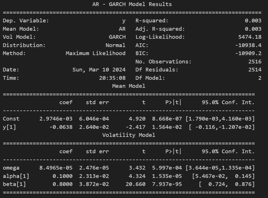
In the regression output we can see that all coefficients are significantly relevant, giving us the following models:


Analyzing results
Aside for looking for significant coefficients (and a high R-squared in the case of ARMA models), we should always look at the residuals when modeling a time series to make sure that all relevant information was captured, and it contains no relevant information.
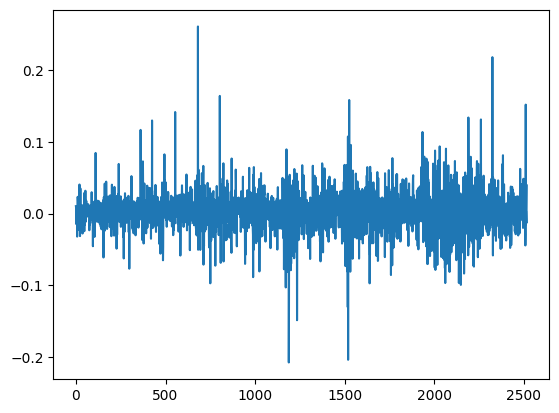
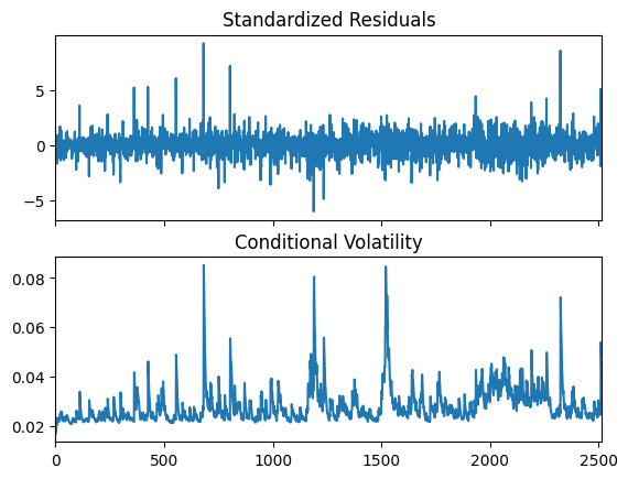
On the left we have the residuals from our AR(1) model, one can easily identify some clustering in the volatility by a simple glance we see that there is a tendency for periods of high volatility to be followed by more periods of high volatility, and periods of low volatility to be followed by more periods of low volatility. The standardized residuals on the right from the AR(1)-GARCH(1,1) model capture the clustering and provides us with a more homoscedastic residual. To finalize our analysis, we will utilize the Ljung-Box test to guarantee that the residuals from our final model are a white noise.
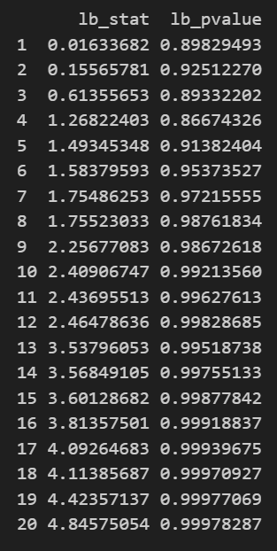
The Ljung-Box test evaluates whether there is significant autocorrelation in a time series’ residuals, crucial for validating the adequacy of a fitted model. The null hypothesis states that there is no autocorrelation present in the residuals, meaning that the residuals are independently and identically distributed (i.i.d.). The alternative hypothesis indicates that autocorrelation exists beyond what random chance would suggest, suggesting that the model may require additional terms or adjustments to capture the remaining temporal dependencies in the data.
The output from the test on the left shows that all p-values are above any typical significance level. Therefore, we cannot reject the null hypothesis and can conclude that the residuals are white noise, indicating a well-fitted model.
Final Thoughts
This article provides the information needed to apply the Generalized Autoregressive Conditional Heteroskedasticity (GARCH) model for analyzing and modeling the volatility dynamics of financial time series data. Implementing the GARCH model allows for effectively capturing the time-varying volatility in financial returns and assessing the impact of past squared errors on current volatility. This methodology helps practitioners better understand and forecast volatility clustering, a crucial aspect of risk management and financial modeling.