
In the ever-changing realm of financial markets, a crucial aspect lies in deciphering the intricate patterns within time series data. Delving into the dynamics of finance, analysts and investors often turn to ARIMA, the Autoregressive Integrated Moving Average model. This robust statistical tool allows one to unravel and forecast the nuanced trends embedded in financial time series, providing a compass for navigating the currents of market movements.
Data
To retrieve our data through the EOD API service, we first need to download and import the EOD Python package, and then authenticate using your personal API key. It’s recommendable to save your API keys in the environment variable. We are going to use the Historical Data API, which is available in our plans. However, some plans have limited time depth (1-30 years).
pip install eodimport os
# load the key from the environment variables
api_key = os.environ['API_EOD']
import eod
client = EodHistoricalData(api_key)1. Use the “demo” API key to test our data from a limited set of tickers without registering:
AAPL.US | TSLA.US | VTI.US | AMZN.US | BTC-USD | EUR-USD
Real-Time Data and all of the APIs (except Bulk) are included without API calls limitations with these tickers and the demo key.
2. Register to get your free API key (limited to 20 API calls per day) with access to:
End-Of-Day Historical Data with only the past year for any ticker, and the List of tickers per Exchange.
3. To unlock your API key, we recommend to choose the subscription plan which covers your needs.
ARIMA (p, d, q)
ARIMA processes can be broken down into 3 main components:
Autoregressive (AR) Component:
The autoregressive part captures the relationship between an observation and its past values. The term “autoregressive” signifies that the model uses past observations as predictors for future values.
Integrated (I) Component:
The integrated part involves differencing the time series data to make it stationary. Stationarity is crucial for many time series models, including ARIMA. Differencing helps in stabilizing the mean and variance of the series. In the case of stock prices, we can use arithmetic or log returns instead of the first difference.
Moving Average (MA) Component:
The moving average component represents the relationship between an observation and a residual error from a moving average model. It captures the short-term fluctuations in the data that are not accounted for by the autoregressive component.
The notation for ARIMA is often represented as ARIMA(p, d, q), where:
- p is the order of the autoregressive component.
- d is the degree of differencing.
- q is the order of the moving average component.
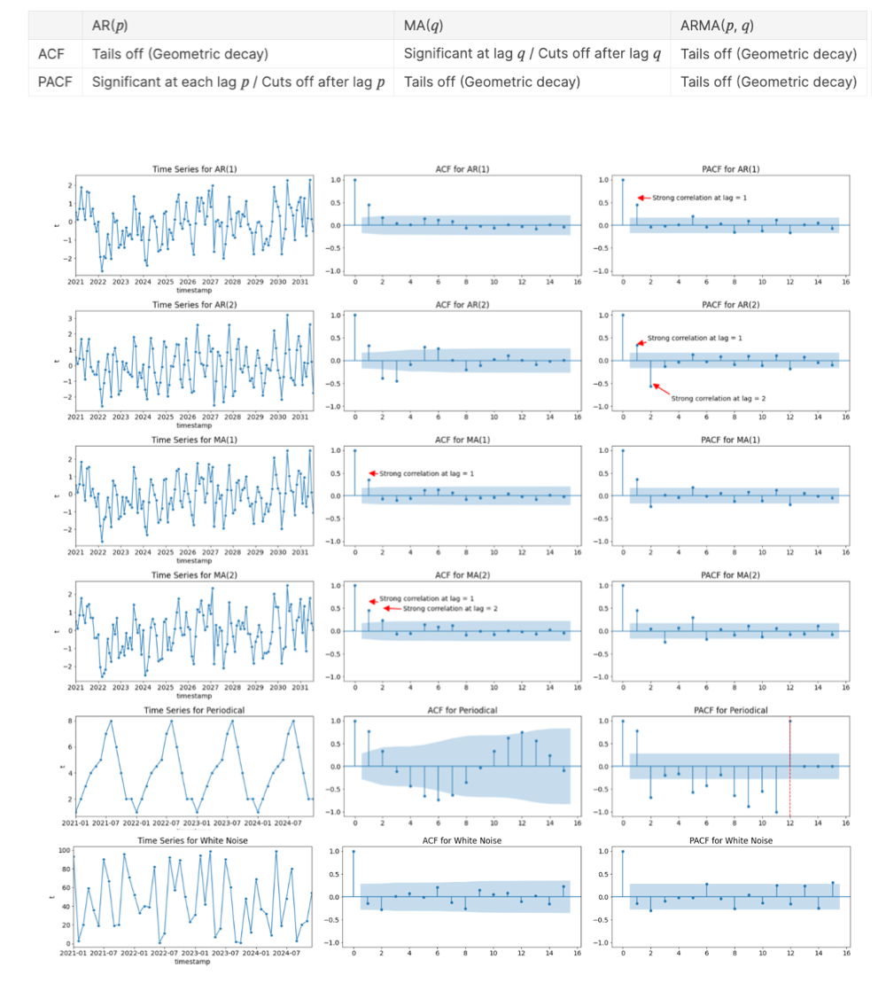
The process of selecting appropriate values for p, d, and q involves analyzing the autocorrelation function (ACF) and partial autocorrelation function (PACF) of the time series data. These functions help identify the presence of autoregressive and moving average components and guide the choice parameters for the model:


are the autoregressive coefficients
is the white noise error term at time t
are the moving average coefficients
Application
Step 1 – Checking for Stationarity
Stationarity is a crucial concept in time series analysis. A stationary time series is one whose statistical properties, such as mean, variance, and autocorrelation, do not change over time. In simpler terms, it exhibits a consistent and stable behavior, making it easier to model and analyze. To check for stationarity one can use a variety of tests such as the Phillips-Perron, KPPS, and the Augmented Dickey-Fuller (ADF). Checking for stationarity involves identifying the presence of a unit root, which represents a coefficient of 1 for the first lagged term (
def ADF(time_series):

    trend_types = ['c', 'ct', 'n']

    for trend in trend_types:
        print(f"Augmented Dickey-Fuller (ADF) test with trend '{trend}':")
        result = sm.tsa.adfuller(time_series, autolag='AIC', regression=trend)
        print(f'ADF Statistic: {result[0]}')
        print(f'p-value: {result[1]}')
        print('Critical Values:')
        for key, value in result[4].items():
            print(f'   {key}: {value}')

        if result[1] <= 0.05:
            print("Reject the null hypothesis; the time series has no unit root.\n")
        else:
            print("Fail to reject the null hypothesis; the time series has a unit root.\n")
In case of failure in rejecting the null hypothesis, the next step would be to take the first difference of the series (d = 1), or in the case of prices, to calculate the returns.
Step 2 – Analyzing the Auto Correlation and Partial Autocorrelation Functions
Once our series becomes stationary, we need to analyze the ACF and PACF to identify the ARMA structure of the process. Many consider this process more art than science, as identifying the orders of p and q can be challenging. That’s why it’s advisable to start from the most complex explanation and test your way into the most parsimonious model. A simpler model with fewer parameters is favored over more complex models with more parameters. To get started, the picture below provides the essentials to identify the order of any ARMA structure and offers a few examples:
The functions below are useful to plot the ACF and PACF during analysis:
def ACF(variable):
    sm.graphics.tsa.plot_acf(variable, lags=20)
    plt.title("ACF")
    plt.show()

def PACF(variable):
    sm.graphics.tsa.plot_pacf(variable, lags=20)
    plt.title("PACF")
    plt.show()
Step 3 – Modeling ARMA(p,q)
Once the orders of p and q have been identified, the following step would be to set up an ARMA(p,q) model. To do so, the code provided below:
import statsmodels.api as sm

p_order = 1 # AR order
q_order = 1 # MA order
d_order = 0 # differencing order

model = sm.tsa.ARIMA(series, order=(p_order, d_order, q_order))
model_fit = model.fit()
print(model_fit.summary())
Step 4 – Interpreting Summary
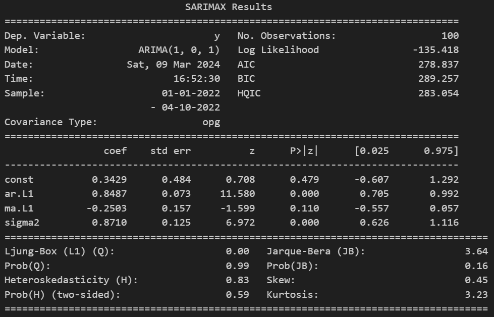
In the sample summary provided, one is able to identify the coefficients for the AR and MA process and judge their efficiency in describing the series according to their respective p-value. In the example provided, it would be interesting to remove the MA part and do a pure AR model due to the p-value above the significance level (1%, 5%, or 10%).
When encountering two reliable models to describe the behavior of the series, it is wise to choose the most parsimonious model and compare models based on the selection criterias such as the Akaike Information Criterion (AIC), Bayesian Information Criterion (BIC) and Hannan-Quinn Information Criterion (HQIC), where the lowest value represents the better fitting model.
Example: NVIDIA stock
To retrieve data, we utilize the Official EOD Python API library. Our process begins with gathering data for NVIDIA dating back to March 2014. Information on stocks is accessible through the use of the get_historical_data function.
start = "2014-03-01"

prices = api.get_historical_data("NVDA", interval="d", iso8601_start=start,
                              iso8601_end="2024-03-01")["adjusted_close"].astype(float)
prices.name = "NVDA"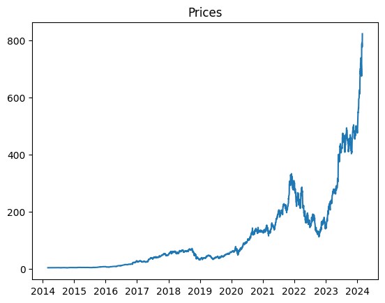
Using the provided code and API, you can fetch the closing prices for the stock and plot them on the left. Upon visual inspection, it’s evident that the data is not stationary. To address this, one should conduct a stationarity test with the ADF-test and identify the type of trend to remove it from the data. Considering prices as random walks, where they are their past value plus some random term, it’s advisable to analyze their returns. This can be achieved with the following code:
Calculating Returns
returns = log(prices/prices.shift(1))[1:]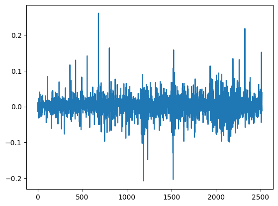
Look how beautiful it is! Now this we can work with. Although there are still some outliers and clustering in the returns, for learning purposes we can proceed to a further analysis on the behavior of NVIDIA’s stock returns.
Autocorrelation and Partial Autocorrelation Functions
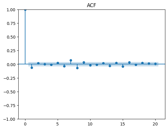
Examining the ACF plot for significant spikes beyond the shaded region, we can identify the presence of a q of order 1 for the MA term. As for the spikes on lag orders 7 and 8, it is possible to build a degenerate model excluding the lags between 1 and 7, but for simplicity and in the search for the most parsimonious model, we will take q with a value of 1.
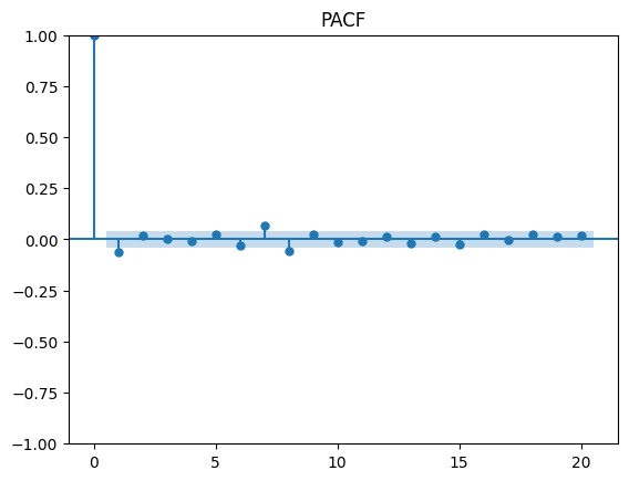
Applying the same process to identify p for the AR term, we can notice a similar pattern and obtain the same result as the one for q.
In conclusion from the observations made we can continue to modeling an ARMA (1,1) process.
Result Summary
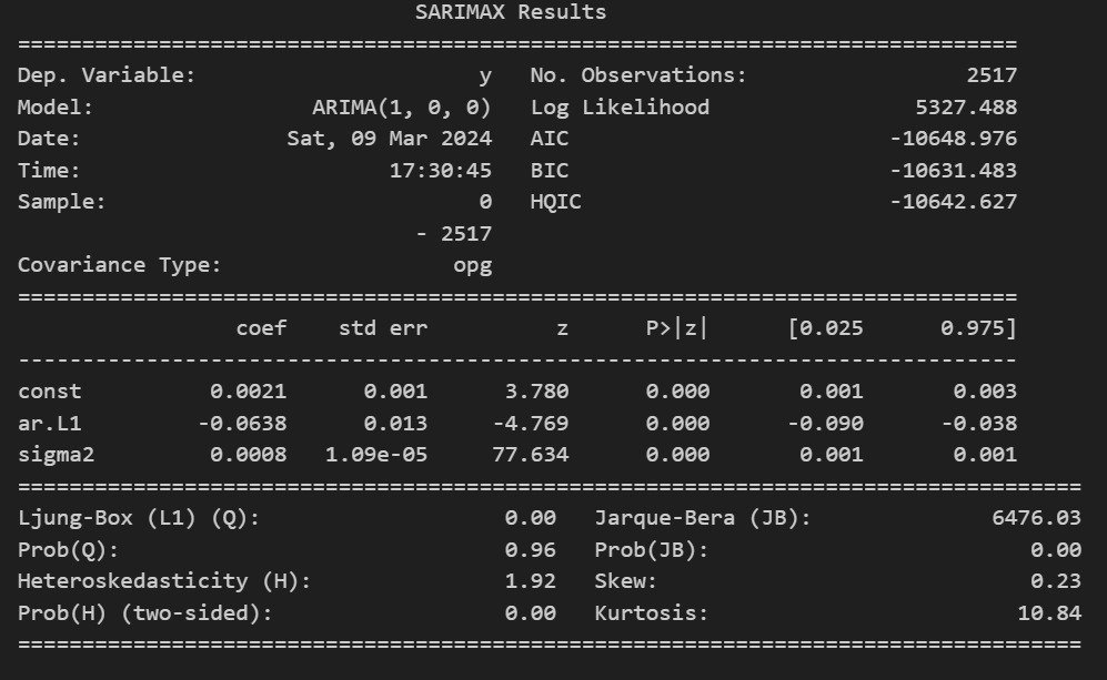
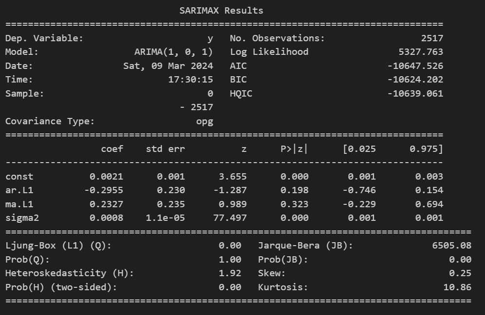
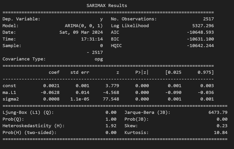
Finding the best fitting model for your time series can be challenging, it is always wise to explore all possibilities before making a decision. On our first attempt, the ARMA(1,1) model, both coefficients for the AR and MA terms are statically insignificant, meaning the model would be better represented without their presence. To extend the analysis, one should test two models, one removing the MA term and another removing only the AR part, as it was done above in the pictures. In both our models, AR(1) and MA(1) the coefficients are statically significant, and both have the same number of parameters. To select a final model, we turn to the selection criteria. The AR(1) process shows a lower value for all three selection criterion meaning it would be the model of choice.
With the information obtained in this article, one should be able to apply the Box–Jenkins method to apply autoregressive moving average (ARMA) or autoregressive integrated moving average (ARIMA) models to find the best fit of a time-series model to past values of a time series.
References:
Full code available here
Website: baglinifinance.com