

A worked example using EODHD data and a self-supervised Transformer for multivariate time-series anomaly detection.
A typical anomaly-detection example in finance looks at a single price series in isolation — a spike, a gap, a sudden jump in volatility. But some of the most useful signals only show up in the relationship between two or more series: two normally co-moving stocks suddenly diverging, a hedge that stops hedging, a spread that breaks its historical pattern.
This post introduces AnomalyBERT, the self-supervised Transformer for multivariate time-series anomaly detection proposed in Jeong et al. (2023), and walks through a small, illustrative application: computing an anomaly-score time series for the pair Coca-Cola (KO) and PepsiCo (PEP), using daily price data pulled through the EODHD Python API.
Quick jump:
What AnomalyBERT actually does
AnomalyBERT is trained without labeled anomalies. Instead, it learns by corrupting its own input: during training, random segments of a time-series window are replaced with one of four synthetic “outlier” patterns — a blended segment, a flattened segment, a lengthened or shortened segment, an injected spike — and the model is trained to recognize which timesteps were corrupted. Because the model never sees real labels, this works on any multivariate series you can supply, with no annotated anomaly dataset required.
Input. A window of multivariate time series

where  is the window length and
 the number of channels. The window is split into patches of consecutive timesteps; a linear embedding layer combines the channels within each patch, and a Transformer encoder then applies self-attention across the sequence of patches (that is, across time).
Output. A per-timestep anomaly score
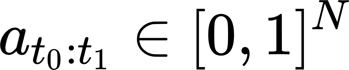
produced by averaging predictions from overlapping sliding windows across the full series. A higher score means the point looked more “corrupted” in the sense the model learned during training — in practice, more unusual relative to the patterns (including the cross-series relationship) that dominate the training data.
Note on pretrained checkpoints. The official implementation ships checkpoints trained on standard industrial benchmarks (SMAP, MSL, SWaT, WADI). Those don’t transfer to financial data — applying the method to a new pair of series, as below, means training your own (small) model on that series.
1. Use the “demo” API key to test our data from a limited set of tickers without registering: AAPL.US | TSLA.US | VTI.US | AMZN.US | BTC-USD | EUR-USD. Real-Time Data and all of the APIs (except Bulk) are included without API calls limitations with these tickers and the demo key.
2. Register to get your free API key (limited to 20 API calls per day) with access to: End-Of-Day Historical Data with only the past year for any ticker, and the List of tickers per Exchange.
3. To unlock your API key, we recommend to choose the subscription plan which covers your needs.
Pulling paired data via the EODHD API
We pull daily adjusted-close prices for KO and PEP going back to 2018, using EODHD’s /eod endpoint. Note that this example needs a subscription plan with full end-of-day history: the demo key covers only a few tickers and the free key only the past year, so neither will work for KO.US and PEP.US from 2018:
import os
import requests
import pandas as pd

def fetch_eod(ticker, start="2018-01-01", end=None):
    token = os.getenv("EODHD_API_TOKEN")
    url = f"https://eodhd.com/api/eod/{ticker}"
    params = {"api_token": token, "period": "d", "fmt": "json", "from": start}
    if end:
        params["to"] = end
    resp = requests.get(url, params=params, timeout=30)
    resp.raise_for_status()
    df = pd.DataFrame(resp.json())
    df["date"] = pd.to_datetime(df["date"])
    return df.set_index("date")

ko  = fetch_eod("KO.US")
pep = fetch_eod("PEP.US")
AnomalyBERT operates on a multivariate matrix, so we build the two-channel input from standardized daily log-returns of both series rather than raw prices — returns are closer to stationary, which matters for a degradation scheme built around detecting deviations from a roughly stable pattern:
import numpy as np

df = pd.DataFrame({"KO": ko["adjusted_close"], "PEP": pep["adjusted_close"]}).dropna()
log_ret = np.log(df / df.shift(1)).dropna()

mu, sigma = log_ret.mean(), log_ret.std()
X = ((log_ret - mu) / sigma).values.astype(np.float32)   # shape (T, 2)
dates = log_ret.index
Building and training the model
The full AnomalyBERT architecture and training pipeline is built for large benchmark datasets and long training runs (up to 150,000 steps in the paper). For an illustrative example like this one, a much smaller version captures the same idea: patch embedding, a shallow Transformer encoder, and a lightweight head producing one anomaly logit per timestep. One simplification worth flagging: the paper injects positional information via a learned relative position bias added to each attention matrix, and explicitly avoids absolute position embeddings; this compact version uses a plain learned absolute positional embedding instead, which is simpler to implement but not what the paper does.
import torch
import torch.nn as nn

PATCH, WINDOW, D_MODEL, N_HEADS, N_LAYERS = 4, 256, 64, 4, 3
N_PATCHES = WINDOW // PATCH

class AnomalyBERTLite(nn.Module):
    def __init__(self, n_channels, patch, d_model, n_heads, n_layers, n_patches):
        super().__init__()
        self.patch = patch
        self.embed = nn.Linear(patch * n_channels, d_model)
        self.pos = nn.Parameter(torch.randn(1, n_patches, d_model) * 0.02)
        enc_layer = nn.TransformerEncoderLayer(
            d_model=d_model, nhead=n_heads, dim_feedforward=4 * d_model,
            dropout=0.1, batch_first=True, activation="gelu")
        self.encoder = nn.TransformerEncoder(enc_layer, num_layers=n_layers)
        self.head = nn.Sequential(nn.Linear(d_model, d_model), nn.GELU(), nn.Linear(d_model, patch))

    def forward(self, x):
        B, T, C = x.shape
        patches = x.reshape(B, T // self.patch, self.patch * C)
        h = self.encoder(self.embed(patches) + self.pos)
        return self.head(h).reshape(B, T)
Training injects one of three synthetic outlier types — a simplified subset of the paper’s four — into random segments of random training windows, and optimizes the model to flag the corrupted timesteps:
def degrade(window):
    w, label = window.copy(), np.zeros(len(window), dtype=np.float32)
    if np.random.rand() < 0.3:
        return w, label  # some windows stay clean
    seg_len = np.random.randint(PATCH * 2, PATCH * 12)
    start = np.random.randint(0, len(w) - seg_len)
    end = start + seg_len
    kind = np.random.choice(["soft_replace", "uniform", "peak"])
    if kind == "soft_replace":
        alt = np.random.randint(0, len(w) - seg_len)
        alpha = np.random.uniform(0.5, 1.0)
        w[start:end] = (1 - alpha) * w[start:end] + alpha * w[alt:alt + seg_len]
    elif kind == "uniform":
        w[start:end] = np.random.uniform(-1, 1, size=(1, w.shape[1]))
    else:
        idx = np.random.randint(start, end)
        w[idx] += np.random.choice([-1, 1]) * np.random.uniform(3, 6)
    label[start:end] = 1.0
    return w, label
Training then samples random windows from the standardized series, degrades each one, and fits the model with a binary cross-entropy loss that up-weights the positive class (pos_weight=5). The seeds are fixed so the run is reproducible; without them, the exact scores — and which dates rank highest — will vary from run to run:
torch.manual_seed(7)
np.random.seed(7)

model = AnomalyBERTLite(X.shape[1], PATCH, D_MODEL, N_HEADS, N_LAYERS, N_PATCHES)

def sample_batch(batch_size):
    xs, ys = [], []
    for _ in range(batch_size):
        start = np.random.randint(0, X.shape[0] - WINDOW)
        w_deg, lbl = degrade(X[start:start + WINDOW])
        xs.append(w_deg)
        ys.append(lbl)
    return (torch.tensor(np.stack(xs), dtype=torch.float32),
            torch.tensor(np.stack(ys), dtype=torch.float32))

N_STEPS, BATCH_SIZE = 800, 32
optim = torch.optim.AdamW(model.parameters(), lr=3e-4)
loss_fn = nn.BCEWithLogitsLoss(pos_weight=torch.tensor(5.0))

model.train()
for step in range(1, N_STEPS + 1):
    xb, yb = sample_batch(BATCH_SIZE)
    loss = loss_fn(model(xb), yb)
    optim.zero_grad()
    loss.backward()
    optim.step()
A few hundred gradient steps is enough for the loss to start flattening out, and by 800 steps — with the positive class up-weighted, since corrupted timesteps are a minority within each window — it’s converged: the full run takes on the order of one to two minutes on a laptop CPU (about 51 seconds in my own run; it varies by machine).
Reading the anomaly score
After training, we slide the model across the full KO/PEP history with a stride shorter than the window, and average the overlapping predictions for each date — the same sliding-window aggregation used in the original paper:
model.eval()
STRIDE = 16
T_full = X.shape[0]
score_sum = np.zeros(T_full, dtype=np.float32)
score_cnt = np.zeros(T_full, dtype=np.float32)

with torch.no_grad():
    for start in range(0, T_full - WINDOW + 1, STRIDE):
        w = X[start:start + WINDOW]
        xb = torch.tensor(w[None, :, :], dtype=torch.float32)
        probs = torch.sigmoid(model(xb)[0]).numpy()
        score_sum[start:start + WINDOW] += probs
        score_cnt[start:start + WINDOW] += 1

valid = score_cnt > 0
anomaly_score = np.full(T_full, np.nan, dtype=np.float32)
anomaly_score[valid] = score_sum[valid] / score_cnt[valid]

result = pd.DataFrame({"KO_close": df["KO"].reindex(dates),
                       "PEP_close": df["PEP"].reindex(dates),
                       "anomaly_score": anomaly_score}, index=dates)
The result is a daily anomaly-score curve alongside the two price series:
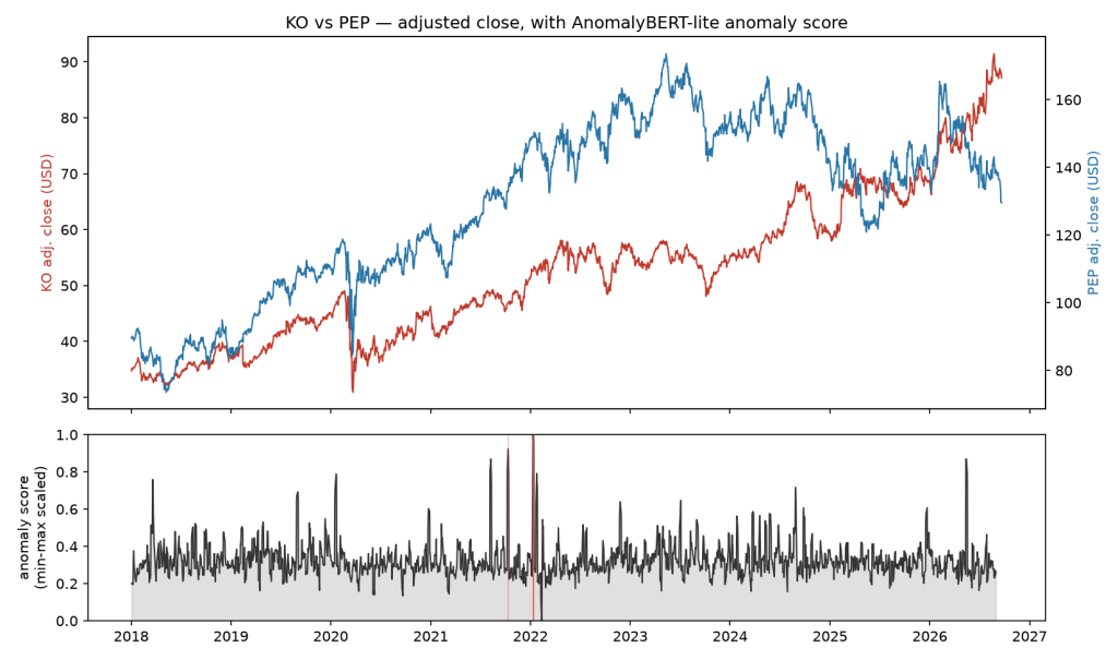
None of the ten highest-scoring dates coincide with either stock’s single largest daily move in isolation — those sit elsewhere in the history entirely. The clearest case of an actual co-movement breakdown is mid-May 2026: the 20-day rolling KO/PEP correlation drops to between its 8th and 15th percentile over the sample, with PEP falling about 1.7% on May 13 against a nearly flat KO. (Those three dates sit at the very tail of the series, though, where sliding-window coverage thins to a third of the usual count, so the scores there are noisier than most.) The other flagged dates — four in January 2022, two in October 2021 and one in August 2021 — don’t show the same clean divergence signature: correlation and returns on those days are unremarkable by comparison. That’s a fair reminder that a small, illustrative model like this one will flag some dates for reasons that don’t reduce to one tidy story; the design intent of a multivariate score over a univariate one — flagging the relationship, not just the level of either series — doesn’t mean every flagged date demonstrates it equally well. All of this refers to data through 21 September 2026; re-running the code later, on a longer sample, will shift the ranking somewhat.
Where this is useful in practice
For a pairs-trading or relative-value setup, a score like this is naturally read as an early-warning or regime-change signal: a spike says “these two, which normally move together, are currently not behaving normally relative to each other” — worth a closer look before sizing or holding a spread position, rather than a buy/sell signal by itself. The same approach extends directly beyond equity pairs — a stock against its sector ETF, two legs of an FX cross, or (closer to some of my own current research) a DEX and CEX funding rate that are supposed to converge.
The categories below describe how a validated score would generally be read in practice — not a verdict on any particular date from the small, illustrative model above, where (as the previous section showed) not every flagged date tells an equally clean story.
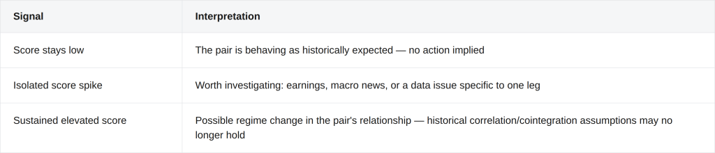
One resolution caveat: every synthetic degradation used in training here — including the single-point “peak noise” type — labels an 8–47-day segment as anomalous, so this particular model isn’t actually trained to tell a true one-day event apart from a multi-day one. Treat the isolated-spike/sustained-elevated split above as a general framework for reading this kind of score, not a distinction this specific model is calibrated to make.
Conclusion
AnomalyBERT’s core contribution — learning to flag anomalies from synthetic self-supervision rather than labeled data — makes it straightforward to apply to a new multivariate series, including financial ones, without an existing anomaly dataset. The example above is deliberately small: a compact model, a short training run, and a well-known, liquid equity pair chosen for clarity rather than realism. Applying this seriously to a real pairs-trading or risk-monitoring workflow would call for a properly tuned architecture, a validation methodology for threshold selection, and testing across a wider set of pairs and regimes than shown here.
A note on the result above. The anomaly score here is sensitive to training hyperparameters — window size, patch size, and how heavily the (rare) synthetic anomaly class is weighted during training all visibly shift which dates score highest. It also has two methodological shortcuts worth flagging: the log-returns are standardized using the mean and standard deviation of the entire series rather than a rolling or expanding window, so later statistics leak slightly into earlier points; and the model is trained and scored on the same data, with no held-out period. Both are fine for a short, illustrative walkthrough like this one, but either would need addressing — rolling standardization and a proper train/test split — before treating the resulting score as a validated signal.
This article is for illustrative and educational purposes only and does not constitute investment advice. The examples are simplified, are based on limited data samples, and have not been validated for trading or risk-management use. Past results do not guarantee future performance. Always conduct independent research, backtest thoroughly, and consult a qualified professional before making investment decisions.
References
- Jeong, Y., Yang, E., Ryu, J. H., Park, I., & Kang, M. (2023). AnomalyBERT: Self-supervised transformer for time series anomaly detection using data degradation scheme. arXiv. https://arxiv.org/abs/2305.04468
- EODHD. (n.d.). EODHD Financial Data APIs [Data set].