Tick, Volume and Dollar Bars in Python with EODHD Tick Data: A Test on SPY

Typically, charts and models in finance look at the market on a clock: one observation every minute, every hour, every day. In Chapter 2 of Advances in Financial Machine Learning, Marcos López de Prado (2018) argues that this is a poor way to sample a market, because information does not arrive at a constant pace. Bars that close after a fixed number of trades, a fixed number of shares or a fixed amount of money traded should sample the market more evenly, and the returns of such bars should be better behaved.

This post puts that claim to a small test. We download 25 trading days of tick data for SPY, the exchange-traded fund that tracks the S&P 500, from 1 September to 6 October 2026 with the EODHD Ticks API (EODHD, n.d.-a), build tick, volume and dollar bars with ordinary time bars as a baseline, and run a reduced version of Exercise 2.1 from the book: four statistical checks on 20 trading days. On the way we meet a practical problem that the book touches only briefly: a few hundred off-exchange trades, printed far from the market and mostly contingent trades, are enough to distort volume and dollar bars badly. We show what they do, what the sl field tells us about them, and how a simple price filter removes them.

Standard Bars in a Nutshell

A bar summarises a stretch of trading by its open, high, low, close and volume. What differs between bar types is the rule that decides when a bar ends.

Time bars end after a fixed amount of clock time, for example every 8 minutes.
Tick bars end after a fixed number of trades.
Volume bars end after a fixed number of shares have traded.
Dollar bars end after a fixed amount of money, price times shares, has traded.

The book calls all four standard bars (Section 2.3.1); the last three sample by activity instead of by the clock. Trading is far from uniform over the day: it is busy at the open and the close and after news, and quiet around lunch. A clock samples the quiet periods as often as the busy ones. Activity-based bars take more samples when much is happening and fewer when little is, which is the intuition behind the claim that their returns are closer to independent and closer to normal.

What We Test: A Reduced Exercise 2.1

Exercise 2.1 of the book works with E-mini S&P 500 futures tick data. Part (a) asks for tick, volume and dollar bars. Part (b) asks for the number of bars per week and which bar type gives the most stable count. Part (c) asks for the serial correlation of returns. Part (d) asks for the variance of returns in every monthly subset and then the variance of those variances. Part (e) asks for the Jarque-Bera normality test. Years of futures ticks with a contract roll are too heavy for a blog post, so we reduce the exercise in four ways.

One instrument: the SPY ETF (ticker SPY.US), which has no futures roll and therefore needs no ETF trick.
One short window: 20 trading days, from 9 September to 6 October 2026, plus 5 earlier trading days that are used only to set the bar sizes.
Daily instead of weekly and monthly subsets: bar counts and return variances are computed for each trading day.
Bars are formed inside each trading day, so that no return spans the overnight gap.

In this post the four checks are called a) to d). They correspond to parts (b) to (e) of the book exercise, while part (a), forming the bars, is the subject of the sections before them.

a) How stable is the daily number of bars?
b) How large is the serial correlation of consecutive returns?
c) How stable is the daily variance of returns?
d) How close to normal are the returns?

Preparations

Create a project folder with its own virtual environment, so that nothing is installed into the global Python, and install the libraries used in this post: numpy, pandas, scipy, matplotlib, pyarrow, requests and python-dotenv.

python -m venv .venv
.venv\Scripts\activate          # Linux/macOS: source .venv/bin/activate
pip install numpy pandas scipy matplotlib pyarrow requests python-dotenv

Keep your EODHD API token in a file named .env next to the scripts, in one line (EODHD_API_TOKEN=your_token), and read it from there. Do not write the token into the code, and do not commit the .env file to a repository.

API Key Activation

1. Use the “demo” API key to test EODHD’s data from a limited set of tickers without registering: AAPL.US | TSLA.US | VTI.US | AMZN.US | BTC-USD | EUR-USD. Real-Time Data and all of the APIs (except Bulk) are included without API call limitations with these tickers and the demo key. Note: SPY.US, used in this example, is not on the demo list, and the US tick data API needs a plan that includes it, so a registered key with that access is required to run the code as it is.
2. Register to get your free API key (limited to 20 API calls per day) with access to End-Of-Day Historical Data with only the past year for any ticker, and the list of tickers per exchange.
3. To unlock your API key, we recommend choosing the subscription plan which covers your needs.

Each request to the Ticks API consumes one API call, and a whole trading session of SPY comes back in a single request, so this post needs one call per trading day.

Downloading SPY Ticks with the EODHD Ticks API

The US tick data API (EODHD, n.d.-a) returns the trades of a US stock or ETF for a time range given in Unix seconds: timestamp in milliseconds, price, size in shares, sequence number, venue code and the sale-conditions field sl, among other fields. If the request sets no limit, the whole time range comes back in one response, and it costs one API call however many rows it holds. SPY trades between 341,748 and 616,305 times in a regular session in our sample, so we ask for each session (9:30 to 16:00 New York time) in one request. A compact version of the logic:

import os
import requests
import pandas as pd
from dotenv import load_dotenv

load_dotenv()                                  # reads EODHD_API_TOKEN from the .env file
TOKEN = os.getenv("EODHD_API_TOKEN")
URL = "https://eodhd.com/api/ticks"

def get_ticks(session, t_from, t_to, ticker="SPY.US"):
    """All ticks in [t_from, t_to] (Unix seconds) in one request; no limit parameter is sent."""
    params = {"api_token": TOKEN, "fmt": "json", "s": ticker, "from": t_from, "to": t_to}
    resp = session.get(URL, params=params, timeout=300)
    resp.raise_for_status()
    return pd.DataFrame(resp.json())           # columns: ts, price, shares, seq, mkt, sub_mkt, sl

Each day is saved as one parquet file, so a repeated run downloads only the days that are missing. Records with zero shares are dropped, and the sale-conditions field sl is kept, because the next section uses it.

Off-Market Prints and How to Filter Them

Our first run on the unfiltered ticks looked wrong. Volume and dollar bars showed a lag-1 autocorrelation of about −0.41, which is far from what one expects from 50 bars a day on a liquid ETF. The reason sits in a handful of trades. Some prints are reported at a price clearly away from the surrounding trades, and some of them are large. A bar closes on the tick that pushes the running total over the bar size, and a large trade is much more likely to be that tick than a small one. The off-market price then becomes the closing price of the bar: the return into that bar contains a spurious jump and the next return jumps back, which is what a negative autocorrelation looks like.

The off-market print filter we use is deliberately simple. A tick is dropped, price and size together, if its price differs by more than 0.25% from the median price of the 201 ticks around it, 100 before and 100 after.

Both numbers are pragmatic choices, not estimated values. A deviation of 0.25% is far outside the normal tick-to-tick noise of SPY, and on the five days we used to test it, the set of removed ticks hardly changed when the window was anywhere between 51 and 1,001 ticks.

def clean_day(day, pct=0.25, window=201):
    """Drop off-market prints from one day of ticks (columns: ts, price, shares)."""
    med = day["price"].rolling(window, center=True, min_periods=1).median()
    dev_pct = 100.0 * (day["price"] - med).abs() / med
    drop = (dev_pct > pct).to_numpy()
    return day.loc[~drop].reset_index(drop=True)

Over the 25 days the filter removes 598 ticks, which is 0.005% of all ticks but 8.99% of all shares traded. On the 20 analysis days alone it removes 519 ticks (0.006%) that carry 9.63% of the shares. The same filter is applied to the warm-up days and to the analysis days. At the end of the post we show the results with and without it.

What are these prints? The venue code and the sale-conditions field sl of the API answer that question. All 598 removed ticks carry the venue code D, which EODHD lists as the FINRA Alternative Display Facility, so they were traded off the exchanges and reported through a FINRA trade reporting facility (596 through the Nasdaq facility and 2 through the NYSE one, according to sub_mkt). They are real trades, not errors in the data. The table splits them by the letters of their sale conditions.

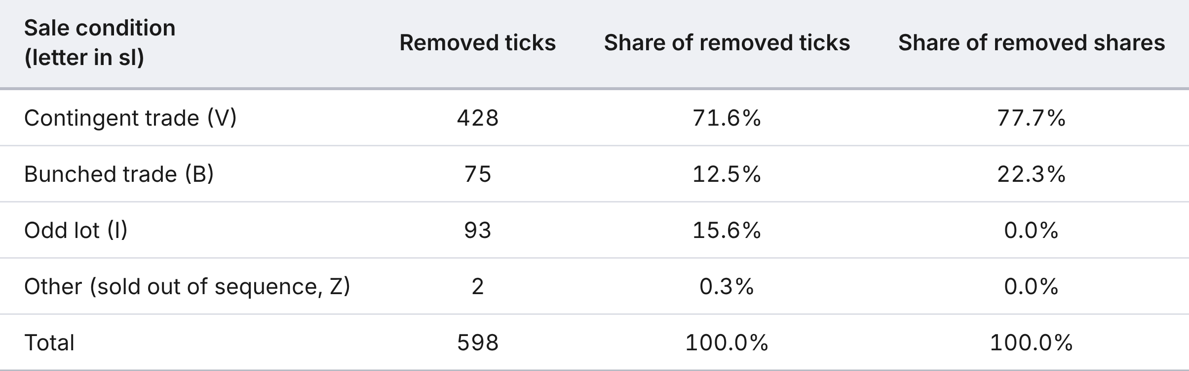
Table of the ticks removed by the filter, split by sale condition: contingent trades, bunched trades, odd lots and other — Notes: The ticks removed by the off-market print filter over the 25 days, grouped by the letters of their sale-conditions field sl; a tick that carries V is counted under V, otherwise under B, otherwise under I. Letter meanings as listed by EODHD (n.d.-a). Source: Author’s own elaboration based on data from EODHD (n.d.-b).

The price rule does not catch every trade of this kind. Over the 25 days, 7,941 ticks carry the condition V, together 11.3% of all shares, and the filter removes 428 of them, the ones that lie furthest from the market.

Forming the Bars

Bars are formed inside each trading day. At 9:30 the running total starts at zero. A bar closes on the first tick that brings the running total to the bar size or above, the closing price is the price of that tick, and the running total then returns to zero. Ticks left over at 16:00 form an unfinished bar, which we drop. The return of a bar is the log change of its closing price from the previous bar of the same day, so the first bar of each day has no return.

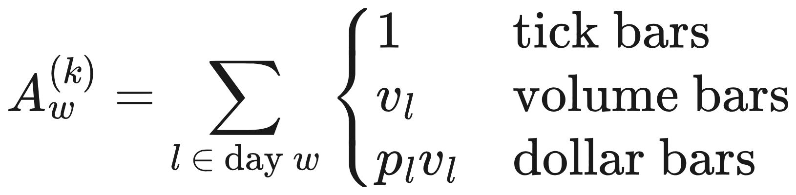
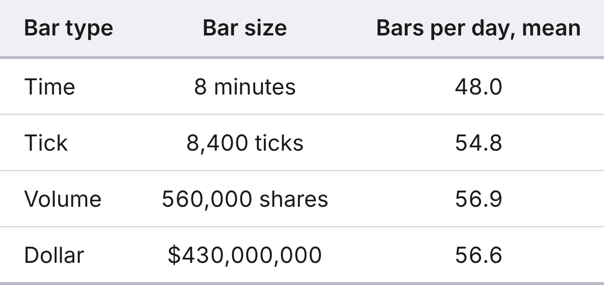
How large should a bar be? We aim at about 50 bars per day for every type. To avoid look-ahead, the bar sizes come only from the five trading days before the analysis window, 1 to 8 September 2026 (7 September was a US holiday). The size is the average daily number of ticks, shares or dollars of those days, divided by 50 and rounded to two significant figures, and it stays fixed for all 20 analysis days. In the formula above, 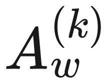is the total traded on warm-up day w, measured in the unit of the bar type: it adds up the same quantity 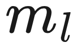as the bar rule, but over all ticks l of that day, so it is the number of ticks for tick bars, the number of shares for volume bars, and the number of dollars (price times shares) for dollar bars. The quantities 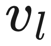and 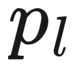are the number of shares and the price of tick l, and 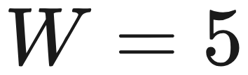is the number of warm-up days. The book uses a constant bar size for standard bars, and so do we. Time bars use 8 minutes, which gives 48 complete bars in a 6.5-hour session.

Table of the four bar types, their fixed bar sizes (8 minutes, 8,400 ticks, 560,000 shares, 430 million dollars) and the mean number of bars per day — Notes: Bar sizes fixed from the five warm-up days, and the resulting number of bars per day on the 20 analysis days. Source: Author’s own elaboration based on data from EODHD (n.d.-b).

def close_indices(measure, T):
    """Index of the tick that closes each bar; the running total restarts at zero."""
    out, acc = [], 0.0
    for i, m in enumerate(measure):
        acc += m
        if acc >= T:
            out.append(i)
            acc = 0.0
    return out

# measure = 1 for every tick (tick bars), shares (volume bars), price * shares (dollar bars)

def bar_size(warmup, bars_per_day=50, sig=2):
    """Average daily activity over the warm-up days divided by the bars per day."""
    n = warmup["date"].nunique()
    activity = {"tick": len(warmup) / n,
                "volume": warmup["shares"].sum() / n,
                "dollar": (warmup["price"] * warmup["shares"]).sum() / n}
    return {k: float(f"{v / bars_per_day:.{sig - 1}e}") for k, v in activity.items()}

Because the bar sizes are fixed, the number of bars per day is not: a busy day produces more bars than a quiet one. Check a) measures exactly this.

Notation for the Four Checks

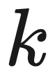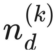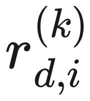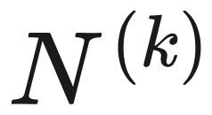
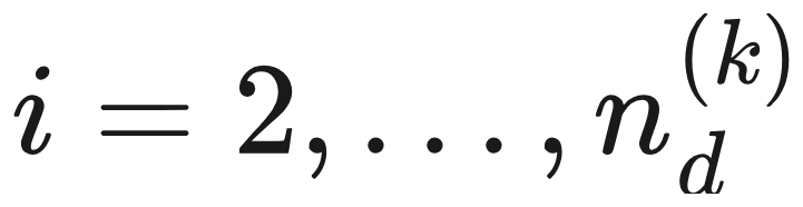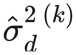
Let = 20 be the number of analysis days and the bar type. On day d, is the number of bars of type k and is the return of its i-th bar, with . All returns of one type together number . The sample variance of the returns of one day is .

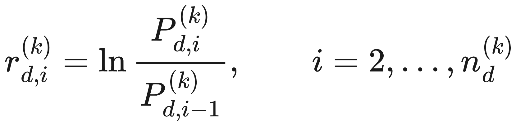
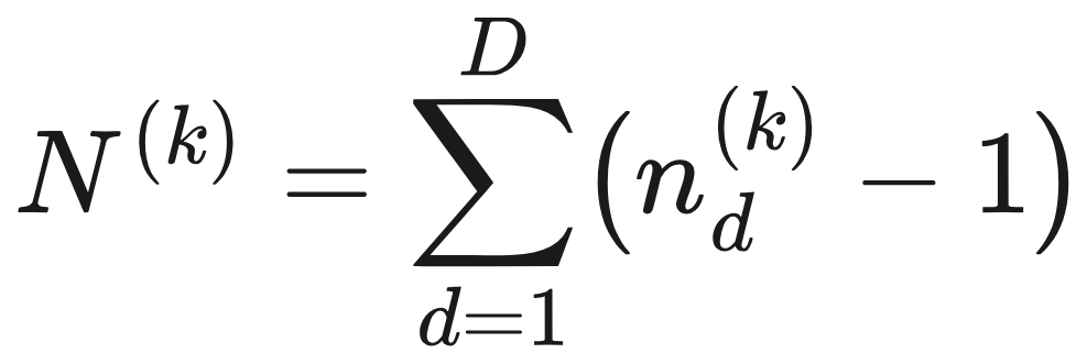
With 20 days, checks a) and c) rest on 20 numbers each. To see how much they could move, we resample the 20 days with replacement 2,000 times, recompute the statistic each time, and report the 2.5th and 97.5th percentiles as a 95% bootstrap interval.

Check a): How Stable Is the Daily Number of Bars?

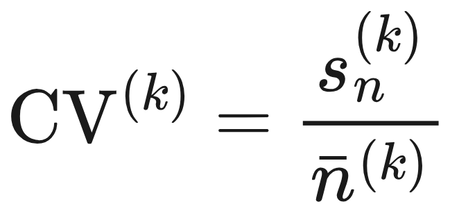
We count the bars on each day, , and compare the spread of the counts across days with their mean. The coefficient of variation 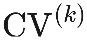is the standard deviation of the daily counts divided by their mean, so a smaller value means a steadier count. Time bars score zero by construction and serve only as a reference.

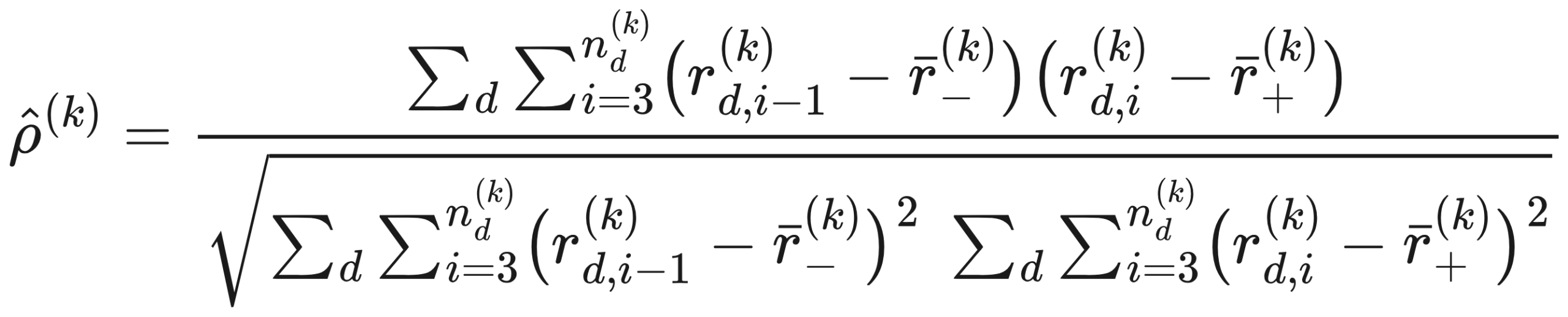
Check b): How Large Is the Serial Correlation of Returns?

We correlate each return with the previous return of the same bar type. Pairs never cross the overnight gap, because the first bar of a day has no return. The correlation is 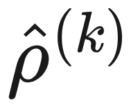, computed over 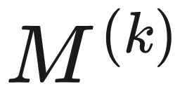pairs, and if returns were independent, about 95% of the values would fall inside 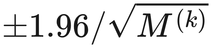. The symbols with a minus and a plus sign below denote the averages of the lagged and of the current returns over all pairs.

Check c): How Stable Is the Daily Variance of Returns?

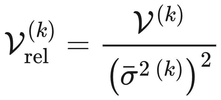
Each day has one variance. If a bar type samples the market in a stable way, its daily variances should be similar from day to day. We take the variance of the 20 daily variances. Because the bar types have different variance scales, we also divide it by the squared mean variance, which gives the scale-free number 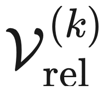that can be compared across types.

Check d): How Close to Normal Are the Returns?

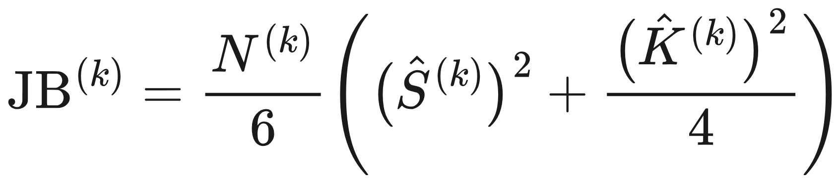
We pool the returns of all days and compute the Jarque-Bera statistic 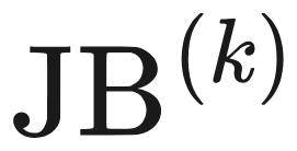from their skewness and excess kurtosis. For normal returns it is close to zero and follows a 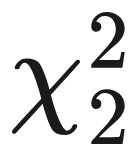distribution, so large values reject normality. As in the book, we use the statistic itself to rank the bar types.

Results

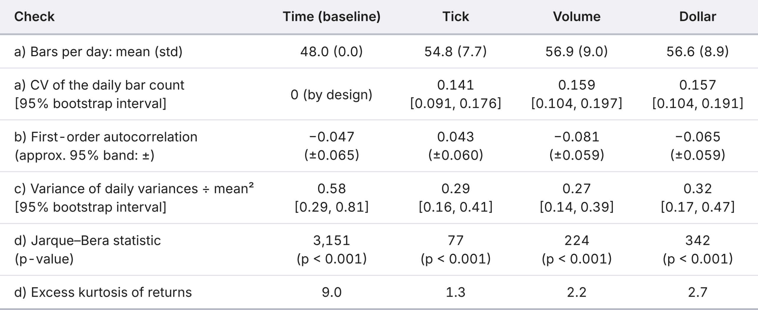
The table collects all four checks. Every statistic is computed on the filtered ticks; the bar sizes are the ones from the table above.

Reading Check a): The Count Is Not Stable

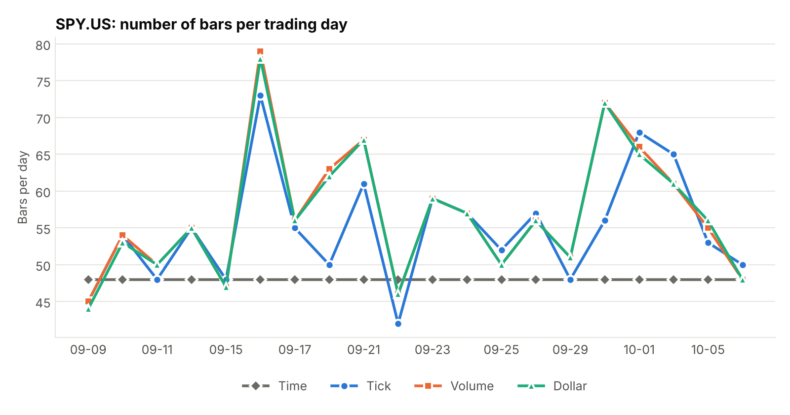
Tick bars have the smallest coefficient of variation (0.141), followed by dollar (0.157) and volume (0.159) bars. The bootstrap intervals overlap almost completely, from 0.09 to 0.20, so 20 days do not separate the three types. More important is what the chart shows: with a fixed bar size, none of the counts is stable. On 16 September, the busiest day of the analysis window with 616,305 ticks, the filtered data gave 73 tick bars and 79 volume bars. On 22 September, the quietest day of the analysis window with 360,983 ticks, it gave 42 tick bars and 46 volume bars. The count follows the day’s activity, and that is what a fixed bar size means.

Line chart of the number of time, tick, volume and dollar bars per trading day for SPY from 9 September to 6 October 2026 — Notes: Bars per trading day. The time-bar count is constant; the three activity-based counts move with the day’s activity. Volume and dollar bar counts are identical on 14 of the 20 days, so the green line covers the orange one. Source: Author’s own elaboration based on data from EODHD (n.d.-b).

Reading Check b): Small Serial Correlation Everywhere

All four estimates are small. Tick bars give 0.043 and time bars −0.047, both inside their 95% bands of about ±0.06. Volume and dollar bars give −0.081 and −0.065, just outside the bands of about ±0.06. By the criterion of the book, the lowest serial correlation, tick bars win, but by a hair, and we would not read much into differences of this size. A small negative value for volume and dollar bars points in the same direction as the off-market effect described above, so part of it may be large prints that survive the filter. We have not tested that.

Reading Check c): The Activity-Based Bars Are Steadier

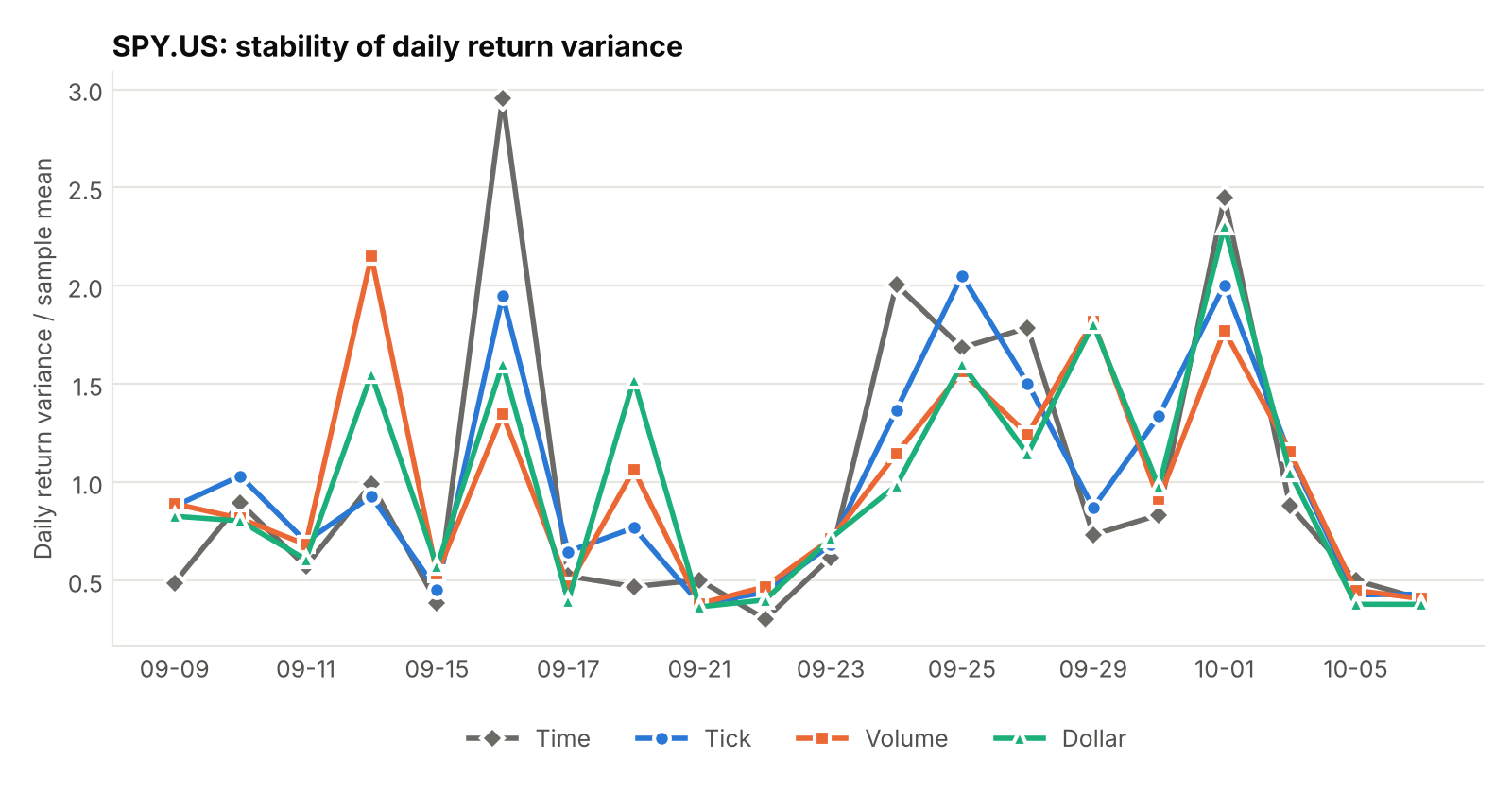
Relative to the squared mean, the variance of the daily variances is 0.58 for time bars, against 0.29 for tick, 0.27 for volume and 0.32 for dollar bars: about half for the three activity-based types, and volume bars come out lowest. The bootstrap intervals overlap (time 0.29 to 0.81, volume 0.14 to 0.39), so with 20 days this is an indication, not a proof. The chart shows where the gap comes from. On 16 September the daily variance of time bars is 2.96 times its sample mean, against 1.95 for tick, 1.60 for dollar and 1.35 for volume bars. All types see the same turbulent days, but the activity-based bars swing less.

Line chart of the daily return variance of time, tick, volume and dollar bars for SPY, each divided by its sample mean — Notes: Daily return variance of each bar type divided by its own sample mean. Source: Author’s own elaboration based on data from EODHD (n.d.-b).

Reading Check d): Closer to Normal, but Not Normal

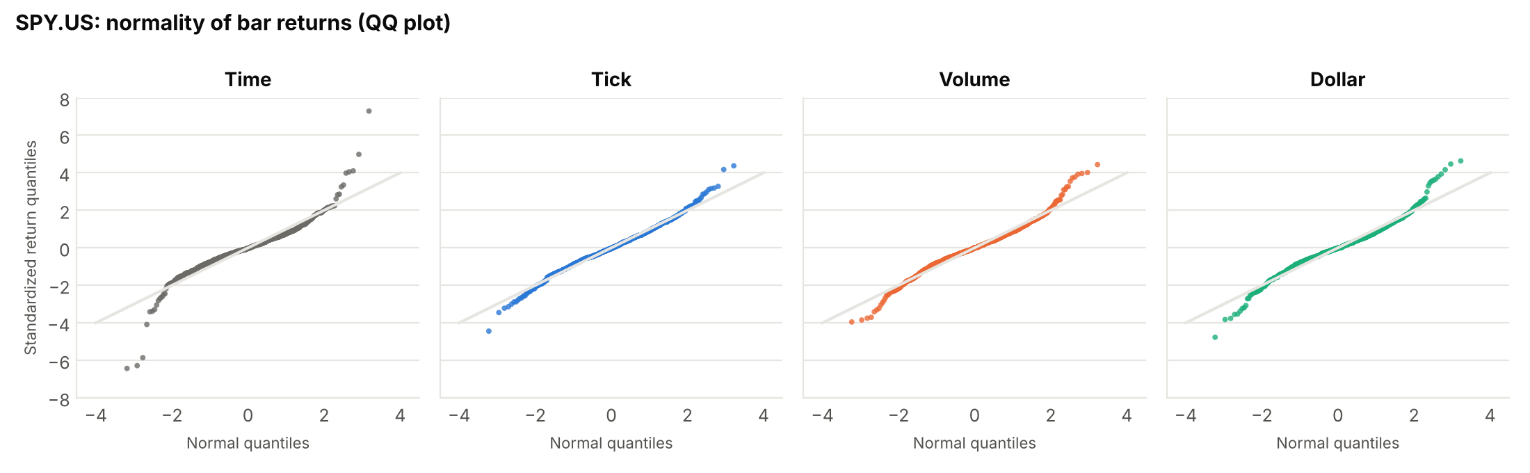
All four types reject normality, with p-values below 10⁻¹⁶, so the ranking matters more than the verdict. Time bars have a Jarque-Bera statistic of 3,151 and an excess kurtosis of 9.0. The activity-based bars are far closer: tick 77 (1.3), volume 224 (2.2) and dollar 342 (2.7). The lowest statistic belongs to tick bars. The QQ plots show the picture: tails are still heavier than normal for every type, but time bars have three returns more than six standard deviations away. Pooling returns across days with different volatility also fattens the tails, so part of the excess kurtosis may come from mixing calm and turbulent days rather than from the bars themselves.

Four normal QQ plots of standardized bar returns for time, tick, volume and dollar bars of SPY — Notes: Normal QQ plots of standardized bar returns, pooled over the 20 days. Source: Author’s own elaboration based on data from EODHD (n.d.-b).

What the Filter Changed

The last table repeats the whole analysis on the raw ticks, including the bar sizes, which are now set from the unfiltered warm-up days: 600,000 shares and $460,000,000 instead of 560,000 shares and $430,000,000, while the tick bar size stays at 8,400 ticks. Time bars are identical in both runs. Tick bars hardly move, because the filter removes only 0.006% of the ticks. Volume and dollar bars change completely: the lag-1 autocorrelation goes from −0.41 and −0.41 to −0.08 and −0.07, the relative variance of variances from 1.37 and 1.69 to 0.27 and 0.32, and the Jarque-Bera statistic from 5,183 and 5,665 to 224 and 342.

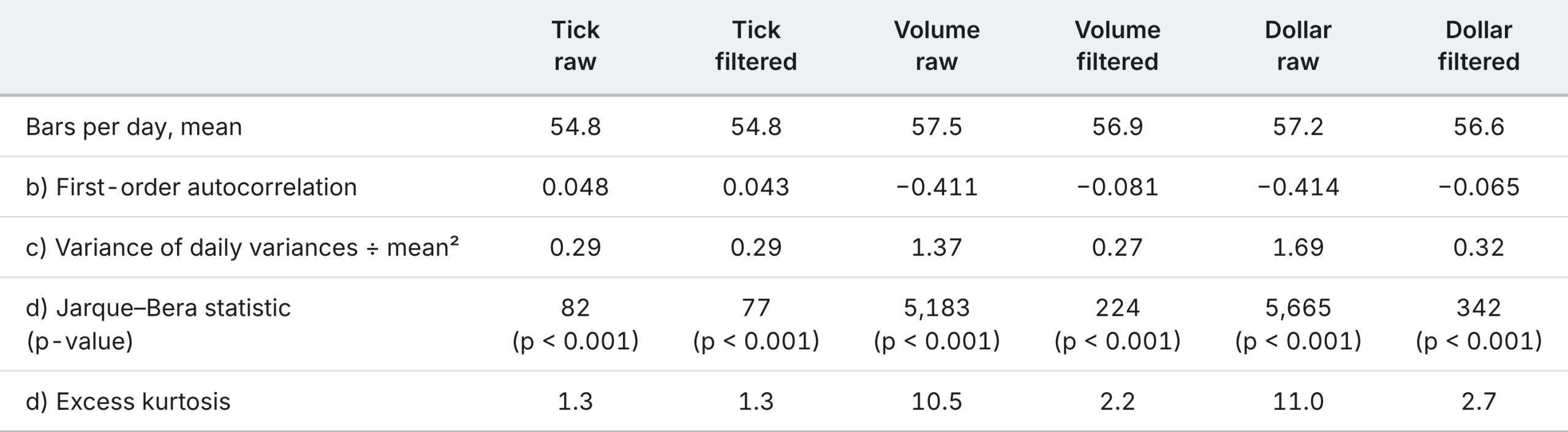
Table comparing tick, volume and dollar bar statistics computed on raw ticks and on filtered ticks — Notes: Tick, volume and dollar bars with and without the off-market print filter (same 20 days; the raw run sets its bar sizes from the unfiltered warm-up days). Time bars are identical in both runs. Source: Author’s own elaboration based on data from EODHD (n.d.-b).

On the raw ticks, volume and dollar bars would look worse than plain time bars on checks b), c) and d), and a reader could conclude that the activity-based bars do not work. With the filter they look better than time bars on c) and d) and comparable on b). In this experiment, the cleaning of the data decided the answer more than the choice of the bar type.

Caveats

These results come from 20 trading days of one ETF, so they illustrate the method rather than settle the question. The bar sizes are static and were set from only five days. The filter parameters are pragmatic choices, and the check of their sensitivity covered only five days. The price filter removes only the contingent trades that lie furthest from the market, so a filter on the sale conditions themselves would remove more, and we did not test its effect. Daily subsets replace the weekly and monthly subsets of the book, and the bootstrap treats days as independent. Finally, the book works with E-mini futures; SPY has a different microstructure, so the numbers are not directly comparable with those in the book.

Conclusion

A reduced version of Exercise 2.1 on 20 days of SPY ticks gives a mixed but useful picture. Activity-based bars do not give a stable number of bars per day, because a fixed bar size follows the activity. They do give a steadier daily variance than time bars, and returns that are far closer to normal, although still not normal. Serial correlation is small for every type. The most practical lesson sits outside the bars themselves: a few hundred off-exchange trades printed far from the market, 0.006% of the ticks, were enough to distort volume and dollar bars, and a simple price filter fixed that. The sl field shows what kind of trades they are, mostly contingent ones. If you build such bars from tick data, inspect the prints before you trust the statistics.

Natural next steps are a longer window and more tickers, a filter on the sale-condition codes instead of the price, and the imbalance and run bars from the next sections of the same chapter.

This post is for illustrative and educational purposes only and does not constitute investment advice. The results come from a short sample and a simple data filter, and they have not been validated for trading or risk-management use. Always conduct independent research and consult a qualified professional before making investment decisions. EODHD does not provide financial advice; data may be subject to delays or inaccuracies as described in EODHD’s terms of use.

References

López de Prado, M. (2018). Advances in Financial Machine Learning. Wiley.
EODHD. (n.d.-a). US Tick Data API documentation.
EODHD. (n.d.-b). EODHD Financial Data APIs [Data set].