

There is an extensive amount of technical indicators out there for trading purposes, but traders being so picky will end up choosing only a handful of them, and the indicator we are going to discuss today definitely adds to this list. Behold the Disparity Index. In this article, we will first discuss what the Disparity Index is all about, the math behind the indicator, and then we will move on to the coding part where we will use Python to first build the indicator from scratch, construct a simple trading strategy based on it, backtest the strategy on the Apple stock and compare the returns to those of the SPY ETF (an ETF designed to track the movements of the S&P 500 market index).
Disparity Index
The Disparity Index is a momentum indicator that measures the distance between the current closing price of a stock and its moving average for a specified number of periods and interprets the readings in the form of percentages. Unlike other momentum oscillators, the Disparity Index is not bound between certain levels and hence is an unbounded oscillator.
Traders often use the Disparity Index to determine the current momentum of a market. Upward momentum in the market can be observed if the readings of the Disparity Index are above zero, and similarly, the market is considered to be in a downward momentum if the readings of the indicator are below zero.
The calculation of the Disparity Index is pretty much straightforward. First, we have to find the difference between the closing of the price of a stock and the moving average for a specified number of periods and divide the difference by the moving average, then multiply it by 100. The calculation of the Disparity Index with a typical setting of 14 as the lookback period can be represented as follows:
DI 14 = [ C.PRICE - MOVING  AVG 14 ] / [ MOVING AVG 14 ] * 100

where,
DI 14 = 14-day Disparity Index
MOVING AVG 14 = 14-day Moving Average
C.PRICE = Closing price of the stock
That’s the whole process of calculating the readings of the Disparity Index. Now, let’s analyze a chart where Apple’s closing price data is plotted along with its 14-day Disparity Index.
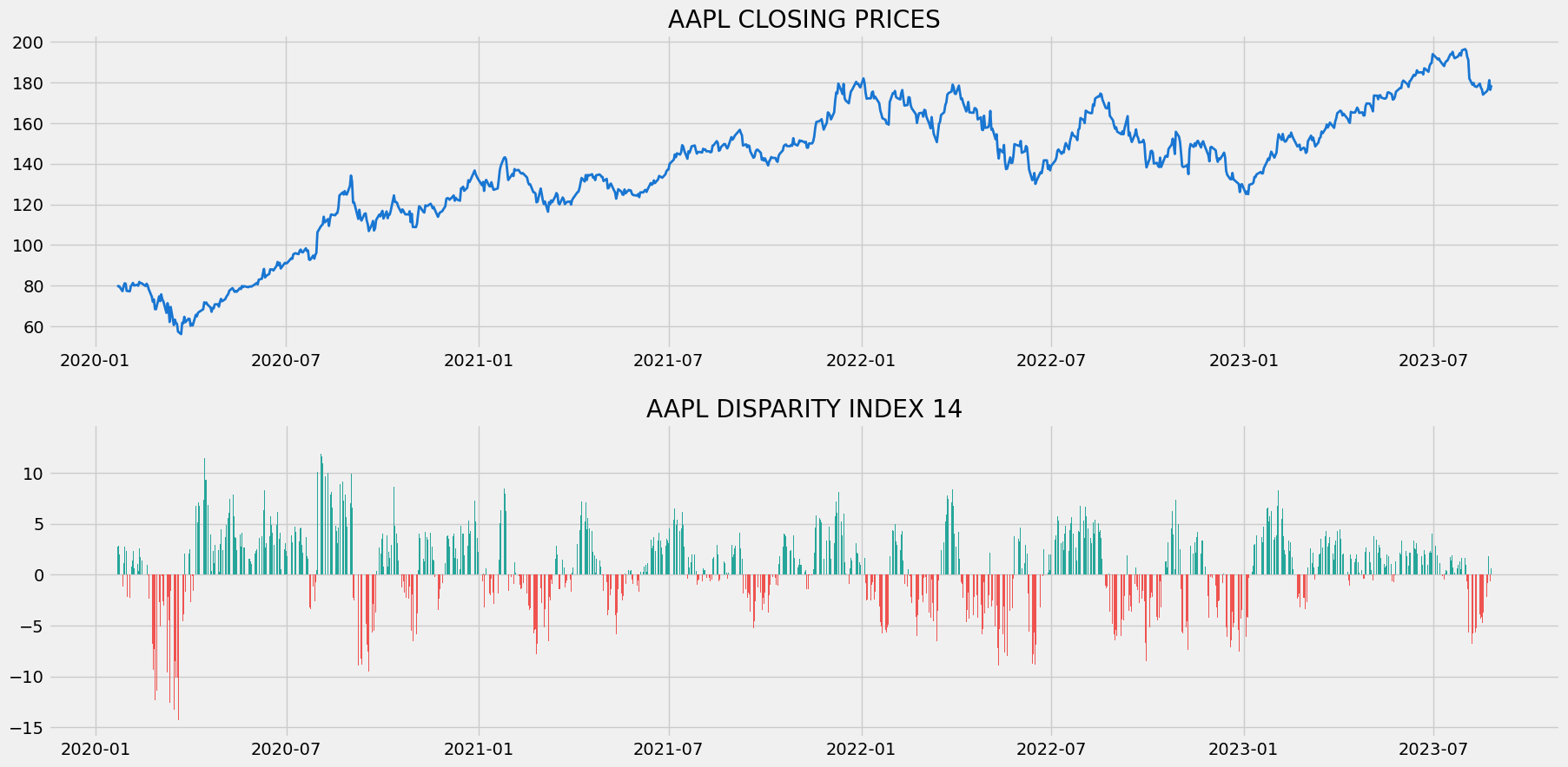
The above chart is separated into two panels: the upper panel with the closing prices of Apple and the lower panel with the readings of the 14-day Disparity Index. From the above chart, we can see that whenever the readings of the Disparity Index are above the zero-line, a green-colored histogram is plotted representing a positive or an upward momentum in the market, and similarly, whenever the Disparity Index goes below the zero-line, a red-colored histogram is plotted representing a negative or downward momentum. This is one way of using the Disparity Index. The other way traders use this indicator is to detect ranging markets (markets where the prices oscillate back and forth between certain limits showing neither positive nor negative price movements). Sometimes, it can be seen that the bars of the Disparity Index go back and forth on either side of the zero line indicating the market is ranging or consolidating. This feature of the indicator comes in handy to traders while making trades (for me personally).
To my knowledge, there are two trading strategies based on the Disparity Index. The first one is the Breakout strategy where traders assume two extreme levels plotted on either side of the plot, and this strategy reveals a buy signal whenever the Disparity Index goes below the lower level, similarly, a sell signal is generated whenever the Disparity Index touches above the upper level. These thresholds vary from one asset to another since the Disparity Index is an unbounded oscillator. The second one is the Zero-line cross strategy which reveals a buy signal whenever the Disparity Index goes from below to above the zero-line, and a sell signal is generated whenever the Disparity Index goes from above to below the zero-line.
In this article, we are going to implement the second strategy which is the Zero-line cross strategy but since the Disparity Index is prone to revealing a lot of false signals, we are going to tune the traditional crossover strategy. Our tuned strategy reveals a buy signal only if the past four readings are below the zero-line and the current reading is above the zero-line. Similarly, a sell signal is generated only if the past four readings are above the zero-line and the current reading is below the zero-line. Doing this would drastically reduce the number of false signals generated by the strategy and thus boost its performance. Our tuned Zero-line crossover trading strategy can be represented as follows:
IF PREV.4 DIs < ZERO-LINE AND CURR.DI > ZERO-LINE ==> BUY SIGNAL
IF PREV.4 DIs > ZERO-LINE AND CURR.DI < ZERO-LINE ==> SELL SIGNAL
This concludes our theory part on the Disparity Index. Now, let’s move on to the programming part where we are first going to build the indicator from scratch, build the tuned Zero-line crossover strategy which we just discussed, then, compare our strategy’s performance with that of SPY ETF in Python. Let’s do some coding! Before moving on, a note on disclaimer: This article’s sole purpose is to educate people and must be considered as an information piece but not as investment advice.
Implementation in Python
The coding part is classified into various steps as follows:
1. Importing Packages
2. Extracting Stock Data from EODHD
3. Disparity Index Calculation
4. Creating the Tuned Zero-line Crossover Trading Strategy
5. Plotting the Trading Lists
6. Creating our Position
7. Backtesting
8. SPY ETF Comparison
We will be following the order mentioned in the above list, so buckle up your seatbelts to follow every upcoming coding part.
Step-1: Importing Packages
Importing the required packages into the Python environment is a non-skippable step. The primary packages are going to be Pandas to work with data, NumPy to work with arrays and for complex functions, Matplotlib for plotting purposes, and Requests to make API calls. The secondary packages are going to be Math for mathematical functions and Termcolor for font customization (optional).
Python Implementation:
# IMPORTING PACKAGES

import numpy as np
import requests
import pandas as pd
import matplotlib.pyplot as plt
from math import floor
from termcolor import colored as cl

plt.style.use('fivethirtyeight')
plt.rcParams['figure.figsize'] = (20,10)
With the required packages imported into Python, we can proceed to fetch historical data for Apple using EODHD’s OHLC split-adjusted data API endpoint.
Step-2: Extracting data from Twelve Data
In this phase, we’re set to retrieve the historical stock data for Apple using the OHLC split-adjusted API endpoint provided by EODHD. It’s important to note that EOD Historical Data (EODHD) is a reliable provider of financial APIs, encompassing an extensive array of market data, including historical data and economic news. Be sure to possess an EODHD account and access your secret API key, a crucial element for data extraction via the API.
Python Implementation:
# EXTRACTING STOCK DATA

def get_historical_data(symbol, start_date):
    api_key = 'YOUR API KEY'
    api_url = f'https://eodhistoricaldata.com/api/technical/{symbol}?order=a&fmt=json&from={start_date}&function=splitadjusted&api_token={api_key}'
    raw_df = requests.get(api_url).json()
    df = pd.DataFrame(raw_df)
    df.date = pd.to_datetime(df.date)
    df = df.set_index('date')
    return df

aapl = get_historical_data('AAPL', '2020-01-01')
aapl.tail()
Output:
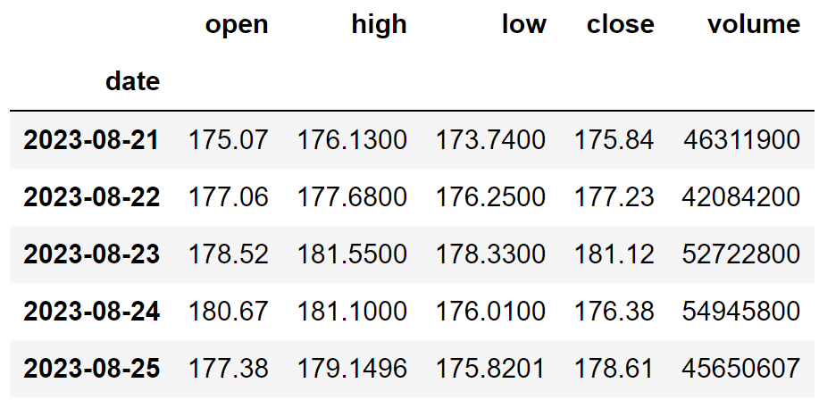
Code Explanation: We begin by defining a function named ‘get_historical_data,’ which takes the stock symbol (‘symbol’) and the start date for historical data (‘start_date’) as parameters. Inside the function, we define the API key and URL, then retrieve the historical data in JSON format using the ‘get’ function and store it in the ‘raw_df’ variable. After cleaning and formatting the raw JSON data, we return it as a Pandas dataframe. Finally, we call this function to fetch Apple’s historical data from the start of 2020 and store it in the ‘aapl’ variable.
Step-3: Disparity Index Calculation
In this step, we are going to calculate the readings of the Disparity Index by following the formula we discussed before.
Python Implementation:
# DISPARITY INDEX CALCULATION

def get_di(data, lookback):
    ma = data.rolling(lookback).mean()
    di = ((data - ma) / ma) * 100
    return di

aapl['di_14'] = get_di(aapl['close'], 14)
aapl = aapl.dropna()
aapl.tail()
Output:
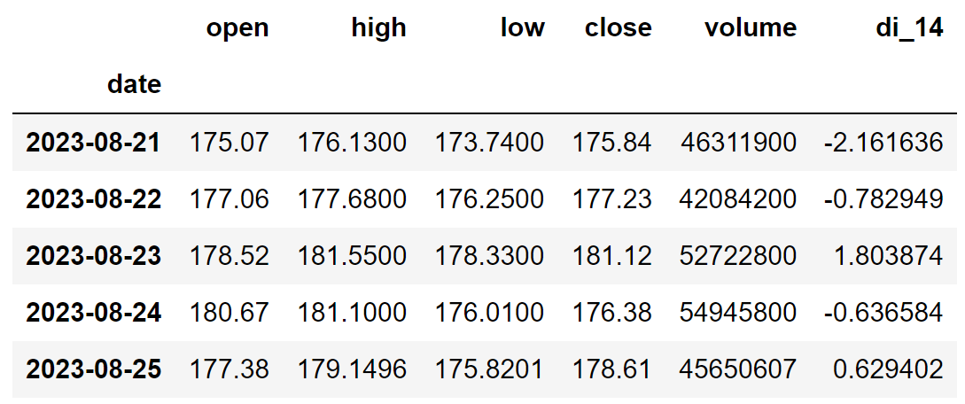
Code Explanation: First, we are defining a function named ‘get_di’ that takes a stock’s closing price (‘data’) and the lookback period as parameters. Inside the function, we are first calculating the Moving Average of the closing price data for a specified number of lookback periods. Then, we substituted the determined values into the Disparity Index formula to calculate the readings. Finally, we are returning and calling the created function to store the 14-day Disparity Index readings of Apple.
Step-4: Creating the trading strategy
In this step, we are going to implement the discussed Disparity Index tuned Zero-line crossover trading strategy in Python.
Python Implementation:
# DISPARITY INDEX STRATEGY

def implement_di_strategy(prices, di):
    buy_price = []
    sell_price = []
    di_signal = []
    signal = 0

    for i in range(len(prices)):
        if di[i-4] < 0 and di[i-3] < 0 and di[i-2] < 0 and di[i-1] < 0 and di[i] > 0:
            if signal != 1:
                buy_price.append(prices[i])
                sell_price.append(np.nan)
                signal = 1
                di_signal.append(signal)
            else:
                buy_price.append(np.nan)
                sell_price.append(np.nan)
                di_signal.append(0)
        elif di[i-4] > 0 and di[i-3] > 0 and di[i-2] > 0 and di[i-1] > 0 and di[i] < 0:
            if signal != -1:
                buy_price.append(np.nan)
                sell_price.append(prices[i])
                signal = -1
                di_signal.append(signal)
            else:
                buy_price.append(np.nan)
                sell_price.append(np.nan)
                di_signal.append(0)
        else:
            buy_price.append(np.nan)
            sell_price.append(np.nan)
            di_signal.append(0)

    return buy_price, sell_price, di_signal

buy_price, sell_price, di_signal = implement_di_strategy(aapl['close'], aapl['di_14'])
Code Explanation: First, we are defining a function named ‘implement_di_strategy’ which takes the stock prices (‘prices’), and the readings of the Disparity Index (‘di’) as parameters.
Inside the function, we are creating three empty lists (buy_price, sell_price, and di_signal) in which the values will be appended while creating the trading strategy.
After that, we are implementing the trading strategy through a for-loop. Inside the for-loop, we are passing certain conditions, and if the conditions are satisfied, the respective values will be appended to the empty lists. If the condition to buy the stock is satisfied, the buying price will be appended to the ‘buy_price’ list, and the signal value will be appended as 1 representing to buy the stock. Similarly, if the condition to sell the stock is satisfied, the selling price will be appended to the ‘sell_price’ list, and the signal value will be appended as -1 representing to sell the stock.
Finally, we are returning the lists appended with values. Then, we call the created function and store the values in their respective variables. The list doesn’t make any sense unless we plot the values. So, let’s plot the values of the created trading lists.
Step-5: Plotting the trading signals
In this step, we are going to plot the created trading lists to make sense of them.
Python Implementation:
# DISPARITY INDEX TRADING SIGNALS PLOT

ax1 = plt.subplot2grid((11,1), (0,0), rowspan = 5, colspan = 1)
ax2 = plt.subplot2grid((11,1), (6,0), rowspan = 5, colspan = 1)
ax1.plot(aapl['close'], linewidth = 2, color = '#1976d2')
ax1.plot(aapl.index, buy_price, marker = '^', markersize = 12, linewidth = 0, label = 'BUY SIGNAL', color = 'green')
ax1.plot(aapl.index, sell_price, marker = 'v', markersize = 12, linewidth = 0, label = 'SELL SIGNAL', color = 'r')
ax1.legend()
ax1.set_title('AAPL CLOSING PRICES')
for i in range(len(aapl)):
    if aapl.iloc[i, 5] >= 0:
        ax2.bar(aapl.iloc[i].name, aapl.iloc[i, 5], color = '#26a69a')
    else:
        ax2.bar(aapl.iloc[i].name, aapl.iloc[i, 5], color = '#ef5350')
ax2.set_title('AAPL DISPARITY INDEX 14')
plt.show()
Output:
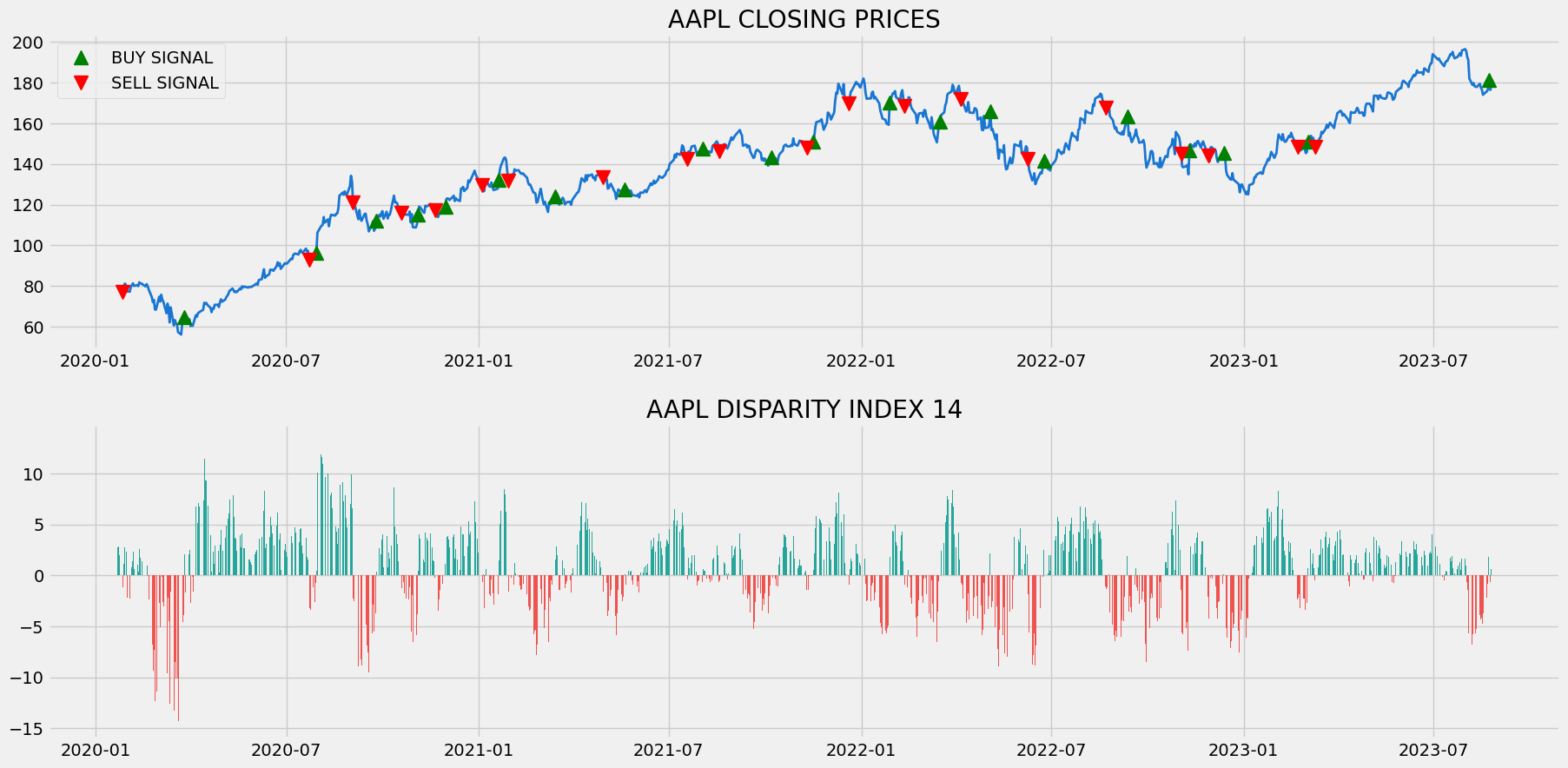
Code Explanation: We are plotting the readings of the Disparity Index along with the buy and sell signals generated by the tuned Zer-line crossover trading strategy. We can observe that whenever the previous four readings of the Disparity Index are below the zero-line and the current reading is above the zero-line, a green-colored buy signal is plotted in the chart. Similarly, whenever the previous four readings of the Disparity Index are above the zero-line and the current reading is below the zero-line, a red-colored sell signal is plotted in the chart.
Step-6: Creating our Position
In this step, we are going to create a list that indicates 1 if we hold the stock or 0 if we don’t own or hold the stock.
Python Implementation:
# STOCK POSITION

position = []
for i in range(len(di_signal)):
    if di_signal[i] > 1:
        position.append(0)
    else:
        position.append(1)

for i in range(len(aapl['close'])):
    if di_signal[i] == 1:
        position[i] = 1
    elif di_signal[i] == -1:
        position[i] = 0
    else:
        position[i] = position[i-1]

close_price = aapl['close']
di = aapl['di_14']
di_signal = pd.DataFrame(di_signal).rename(columns = {0:'di_signal'}).set_index(aapl.index)
position = pd.DataFrame(position).rename(columns = {0:'di_position'}).set_index(aapl.index)

frames = [close_price, di, di_signal, position]
strategy = pd.concat(frames, join = 'inner', axis = 1)

strategy.head()
Output:
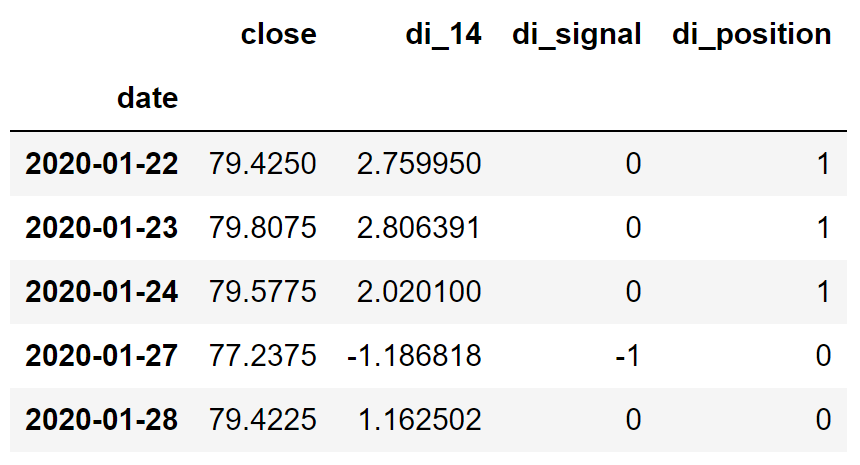
Code Explanation: First, we are creating an empty list named ‘position’. We are passing two for-loops, one is to generate values for the ‘position’ list to just match the length of the ‘signal’ list. The other for-loop is the one we are using to generate actual position values. Inside the second for-loop, we are iterating over the values of the ‘signal’ list, and the values of the ‘position’ list get appended concerning which condition gets satisfied. The value of the position remains 1 if we hold the stock or remains 0 if we sold or don’t own the stock. Finally, we are doing some data manipulations to combine all the created lists into one dataframe.
From the output being shown, we can see that in the first three rows, our position in the stock has remained 1 (since there isn’t any change in the Disparity Index signal) but our position suddenly turned to -1 as we sold the stock when the Disparity Index trading signal represents a sell signal (-1). Our position will remain 0 until some changes in the trading signal occur. Now it’s time to implement some backtesting process!
Step-7: Backtesting
Before moving on, it is essential to know what backtesting is. Backtesting is the process of seeing how well our trading strategy has performed on the given stock data. In our case, we are going to implement a backtesting process for our Disparity Index trading strategy over the Apple stock data.
Python Implementation:
# BACKTESTING

aapl_ret = pd.DataFrame(np.diff(aapl['close'])).rename(columns = {0:'returns'})
di_strategy_ret = []

for i in range(len(aapl_ret)):
    returns = aapl_ret['returns'][i]*strategy['di_position'][i]
    di_strategy_ret.append(returns)

di_strategy_ret_df = pd.DataFrame(di_strategy_ret).rename(columns = {0:'di_returns'})
investment_value = 100000
di_investment_ret = []

for i in range(len(di_strategy_ret_df['di_returns'])):
    number_of_stocks = floor(investment_value/aapl['close'][i])
    returns = number_of_stocks*di_strategy_ret_df['di_returns'][i]
    di_investment_ret.append(returns)

di_investment_ret_df = pd.DataFrame(di_investment_ret).rename(columns = {0:'investment_returns'})
total_investment_ret = round(sum(di_investment_ret_df['investment_returns']), 2)
profit_percentage = floor((total_investment_ret/investment_value)*100)
print(cl('Profit gained from the DI strategy by investing $100k in aapl : {}'.format(total_investment_ret), attrs = ['bold']))
print(cl('Profit percentage of the DI strategy : {}%'.format(profit_percentage), attrs = ['bold']))
Output:
Profit gained from the DI strategy by investing $100k in AAPL : 105467.66
Profit percentage of the DI strategy : 105%
Code Explanation: First, we are calculating the returns of the Apple stock using the ‘diff’ function provided by the NumPy package and we have stored it as a dataframe in the ‘aapl_ret’ variable. Next, we are passing a for-loop to iterate over the values of the ‘aapl_ret’ variable to calculate the returns we gained from our Disparity Index trading strategy, and these returns values are appended to the ‘di_strategy_ret’ list. Next, we are converting the ‘di_strategy_ret’ list into a dataframe and storing it into the ‘di_strategy_ret_df’ variable.
Next comes the backtesting process. We are going to backtest our strategy by investing a hundred thousand USD into our trading strategy. So first, we are storing the amount of investment into the ‘investment_value’ variable. After that, we are calculating the number of Apple stocks we can buy using the investment amount. You can notice that I’ve used the ‘floor’ function provided by the Math package because, while dividing the investment amount by the closing price of Apple stock, it spits out an output with decimal numbers. The number of stocks should be an integer but not a decimal number. Using the ‘floor’ function, we can cut out the decimals. Remember that the ‘floor’ function is way more complex than the ‘round’ function. Then, we are passing a for-loop to find the investment returns followed by some data manipulation tasks.
Finally, we are printing the total return we got by investing a hundred thousand into our trading strategy and it is revealed that we have made an approximate profit of one hundred and five thousand USD in one year. That’s not bad at all! Now, let’s compare our returns with SPY ETF (an ETF designed to track the S&P 500 stock market index) returns.
Step-8: SPY ETF Comparison
While this step is optional, it is highly recommended as it enables us to assess the performance of our trading strategy against a benchmark (SPY ETF). Here, we’ll extract SPY ETF data using the ‘get_historical_data’ function and compare the returns from the SPY ETF with the returns generated by our trading strategy applied to Apple stock.
Python Implementation:
# SPY ETF COMPARISON

def get_benchmark(start_date, investment_value):
    spy = get_historical_data('SPY', start_date)['close']
    benchmark = pd.DataFrame(np.diff(spy)).rename(columns = {0:'benchmark_returns'})

    investment_value = investment_value
    benchmark_investment_ret = []

    for i in range(len(benchmark['benchmark_returns'])):
        number_of_stocks = floor(investment_value/spy[i])
        returns = number_of_stocks*benchmark['benchmark_returns'][i]
        benchmark_investment_ret.append(returns)

    benchmark_investment_ret_df = pd.DataFrame(benchmark_investment_ret).rename(columns = {0:'investment_returns'})
    return benchmark_investment_ret_df

benchmark = get_benchmark('2020-01-01', 100000)
investment_value = 100000
total_benchmark_investment_ret = round(sum(benchmark['investment_returns']), 2)
benchmark_profit_percentage = floor((total_benchmark_investment_ret/investment_value)*100)
print(cl('Benchmark profit by investing $100k : {}'.format(total_benchmark_investment_ret), attrs = ['bold']))
print(cl('Benchmark Profit percentage : {}%'.format(benchmark_profit_percentage), attrs = ['bold']))
print(cl('DI Strategy profit is {}% higher than the Benchmark Profit'.format(profit_percentage - benchmark_profit_percentage), attrs = ['bold']))
Output:
Benchmark profit by investing $100k : 40344.61
Benchmark Profit percentage : 40%
DI Strategy profit is 65% higher than the Benchmark Profit
Code Explanation: The code used in this step is almost similar to the one used in the previous backtesting step but, instead of investing in Apple, we are investing in SPY ETF by not implementing any trading strategies. From the output, we can see that our Disparity Index tuned zero-line crossover trading strategy has outperformed the SPY ETF by 65%. That’s great!
Final Thoughts!
After an exhaustive process of crushing both theory and programming parts, we have successfully learned what the Disparity Index is all about, the mathematics behind it, and finally, how to build the indicator from scratch and construct a tuned zero-line crossover trading strategy based on it with Python. Even though we managed to build a strategy that makes a profit, there are still a lot of spaces where this article can be improved and one such important space is constructing a more realistic strategy.
The procedures, steps, and code we implemented in this article can be suitable for virtual trading but the real-world market doesn’t behave the same way and to thrive in such conditions, it is essential to build our strategy by considering more external factors like risks involved in each trade, commission or fees charged for each transaction, and most importantly market sentiment.
The process isn’t finished even after building a realistic strategy, but it is necessary to know whether the strategy is even a profitable one or just a waste of time. In order to determine the profitability and the performance of the strategy, one has to backtest and evaluate it with various metrics. And this would be the next space where the article can be improved.
If you’re done with these improvisations, you’re set to apply them in the real-world market and the certainty of you being profitable is high. With that being said, you’ve reached the end of the article. Hope you learned something new and useful from this article.