

Technical indicators have become commonplace in the trading world, and dedicating time to studying them is well worth it. While these indicators hold immense potential for market analysis, it’s crucial to acknowledge their limitations. One notable drawback is their tendency to generate false signals, which can lead to disastrous outcomes when followed blindly. While avoiding such signals can be challenging, it’s not impossible, and one effective approach is combining two technical indicators. By doing so, one indicator acts as a filter, distinguishing genuine signals from false ones. This strategy forms the core of our discussion today.
In this article, we will merge two potent technical indicators, namely Williams %R and Moving Average Convergence/Divergence (MACD), to craft a robust trading strategy. The goal is to minimize the impact of false trading signals and substantially enhance investment returns. Without further delay, let’s delve into the heart of this article.
Williams %R
Developed by Larry Williams, the Williams %R stands as a momentum indicator with values ranging from 0 to -100. While sharing similarities with the Stochastic Oscillator, it distinguishes itself through its calculation method. Traders employ this indicator to identify potential entry and exit points for trades by establishing overbought and oversold levels. Before delving into these terms, let’s clarify: a stock is labeled as overbought when market trends are exceptionally bullish and likely to consolidate. Conversely, a stock enters an oversold territory when market trends are exceedingly bearish and exhibit potential for a rebound. While the conventional overbought and oversold thresholds are 20 and 80, respectively, there’s flexibility to explore other values as well.
Calculating Williams %R values within the standard setting of a 14-day lookback period involves several steps. First, the highest high and lowest low for each period over a fourteen-day interval are identified. Subsequently, two differences are computed: the closing price subtracted from the highest high, and the lowest low subtracted from the highest high. Finally, the initial difference is divided by the second difference, and the result is multiplied by -100 to yield the Williams %R values. This calculation can be expressed mathematically as follows:
W%R 14 = [ H.HIGH - C.PRICE ] / [ L.LOW - C.PRICE ] * ( - 100 )

where,
W%R 14 = 14-day Williams %R of the stock
H.HIGH = 14-day Highest High of the stock
L.LOW = 14-day Lowest Low of the stock
C.PRICE = Closing price of the stock
The fundamental concept behind this indicator is rooted in the notion that in a robust uptrend, a stock will continually achieve new highs, while in a substantial downtrend, it will consistently hit new lows. To solidify our grasp of the indicator, let’s examine a Williams %R chart and delve deeper into its dynamics.
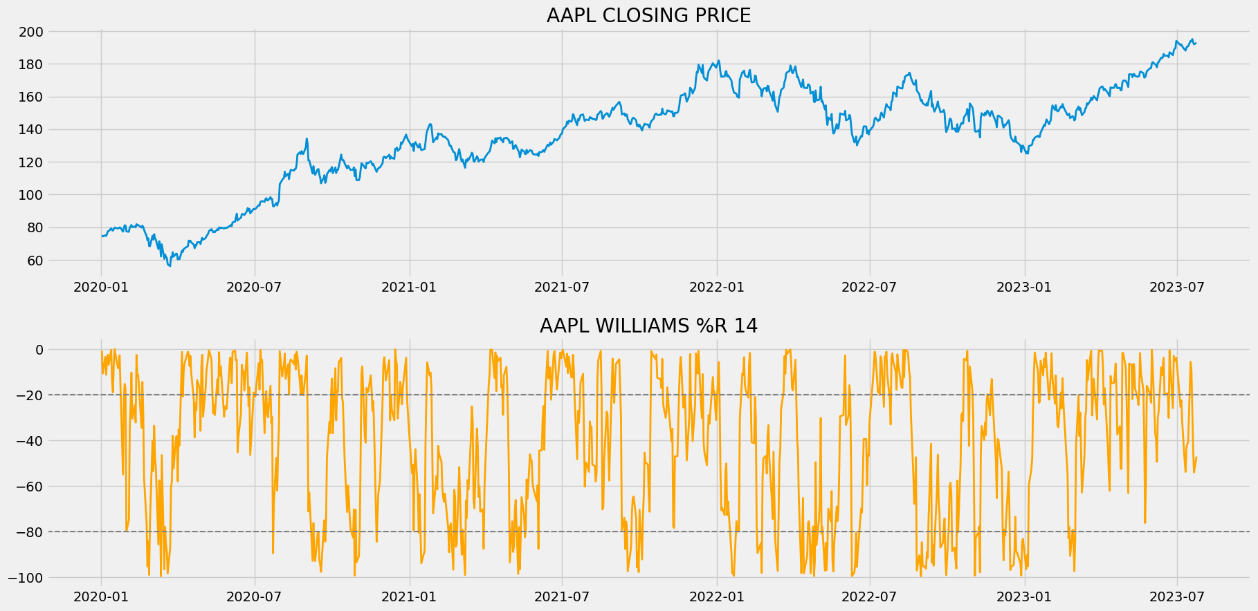
The chart displayed above comprises two panels: The upper panel showcases the closing prices of Apple’s stock data, while the lower panel illustrates the 14-day Williams %R readings for Apple. This chart can be harnessed in two distinct ways.
The first approach involves utilizing the chart as a tool to recognize overbought and oversold conditions within the market. Notice the presence of two horizontal grey lines plotted above and below the market. These lines denote the overbought and oversold levels, set at thresholds of -20 and -80, respectively. If the Williams %R reading surpasses the upper line (overbought line), it suggests an overbought market state. Conversely, if the reading falls below the lower line (oversold line), it indicates an oversold market condition.
The second approach to employing Williams %R is to identify false momentum in the market. During robust uptrends, the Williams %R readings frequently exceed -20. However, if the indicator’s reading drops and struggles to surpass -20 before declining again, this signals inauthentic momentum and the possibility of a significant downtrend. Similarly, during healthy downtrends, the Williams %R readings tend to frequently dip below -80. Should the indicator’s reading rise and fail to reach -80 before the next ascent, it implies an impending positive trend.
Given that Williams %R is a directional indicator (an indicator whose movement is directly proportional to that of the actual market), traders also employ it to identify and validate strong uptrends or downtrends in the market, allowing them to trade in alignment with these trends. Unlike some indicators that might lag in nature (taking past data points into account to determine the present reading), Williams %R is effective due to its status as a leading indicator (considering previous data points to predict future movements).
MACD
Before delving into the details of MACD, it’s crucial to understand the concept of Exponential Moving Average (EMA). EMA is a type of Moving Average (MA) that assigns higher weight (or importance) to the most recent data point while assigning relatively lower weight to data points further in the past. To illustrate, consider a question paper comprising 10% one-mark questions, 40% three-mark questions, and 50% long answer questions. This analogy demonstrates how distinct weights are assigned to different sections of the question paper based on their significance (where long answer questions hold more weight than one-mark questions).
Now, let’s turn our attention to MACD. MACD stands for Moving Average Convergence/Divergence, and it functions as a trend-following leading indicator. The MACD value is calculated by subtracting two Exponential Moving Averages (EMAs), one with a longer period and the other with a shorter period. There are three prominent components within a MACD indicator.
- MACD Line: This component represents the disparity between two distinct Exponential Moving Averages (EMAs). To compute the MACD line, two EMAs are calculated: one with a longer period, referred to as the slow length, and another with a shorter period, known as the fast length. Common choices for the fast and slow lengths are 12 and 26, respectively. The ultimate MACD line values are obtained by subtracting the slow length EMA from the fast length EMA. The formula for calculating the MACD line can be expressed as follows:
MACD LINE = FAST LENGTH EMA - SLOW LENGTH EMA
- Signal Line: This component represents the Exponential Moving Average (EMA) of the MACD line over a specified period. The most commonly used period for calculating the Signal line is 9. Since we’re averaging the MACD line itself, the Signal line tends to exhibit smoother behavior compared to the MACD line.
- Histogram: As implied by its name, the histogram is a visual representation that discloses the distinction between the MACD line and the Signal line. This histogram proves valuable for trend identification. The formula for computing the Histogram can be articulated as follows:
HISTOGRAM = MACD LINE - SIGNAL LINE
Now that we’ve established a comprehensive understanding of MACD, let’s proceed to analyze a MACD chart. This analysis will help solidify our intuitive grasp of the indicator’s behavior and dynamics.
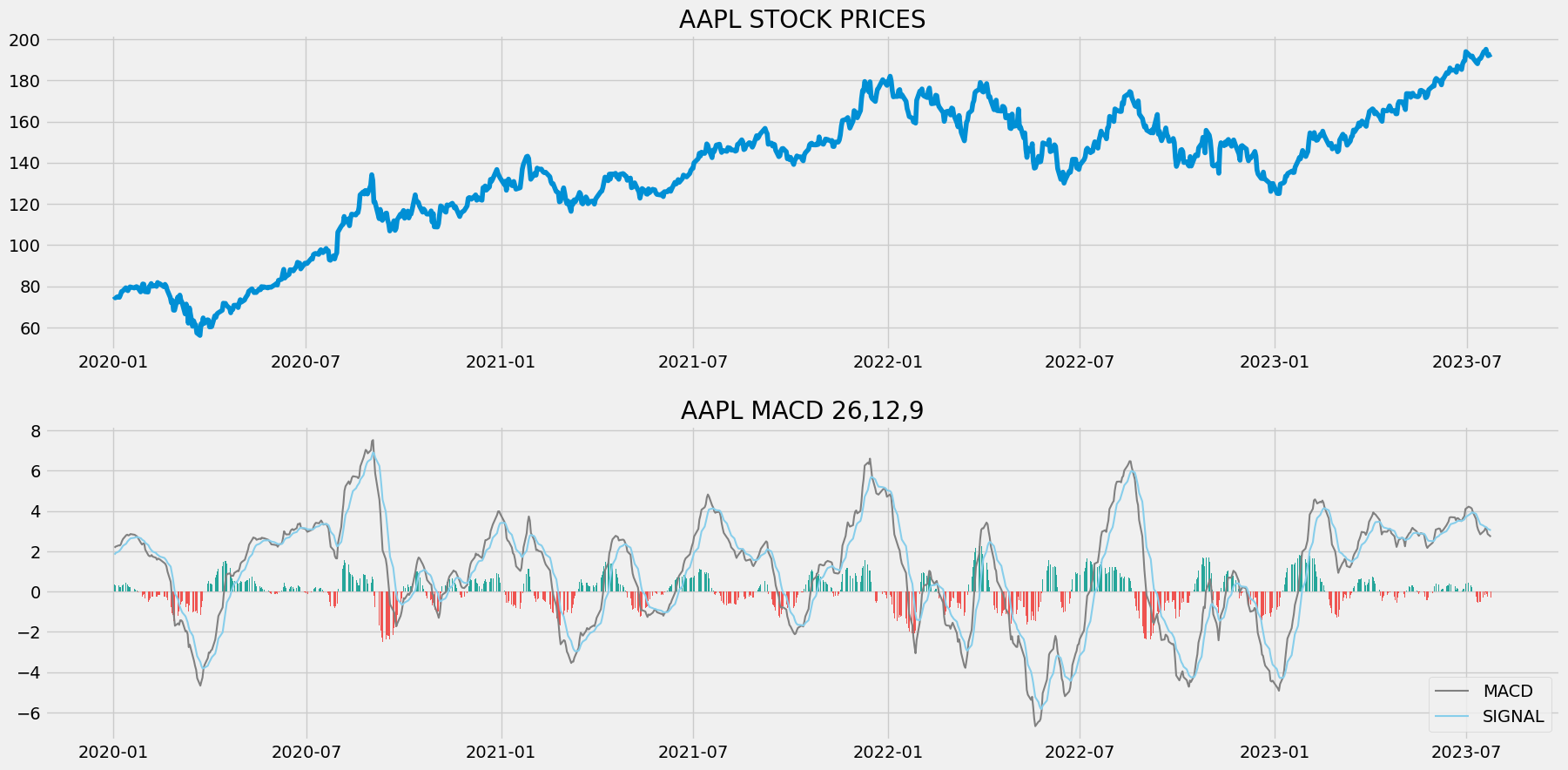
In the plotted chart, two panels are presented: the upper panel displays Apple’s closing prices, while the lower panel showcases a series of plots illustrating the calculated components of MACD. Let’s examine each component in detail.
The most prominent and conspicuous element within the lower panel is undoubtedly the plot of Histogram values. Notice that this plot turns red when the market trend is negative and shifts to green when the market trend is positive. This attribute of the Histogram plot proves exceptionally useful for identifying the prevailing market trend. The Histogram plot expands significantly when the gap between the MACD line and the Signal line is substantial. Conversely, it contracts during periods when the difference between these two components is relatively smaller.
The following two components are the MACD line and the Signal line. The MACD line, depicted in grey, showcases the disparity between the slow-length Exponential Moving Average (EMA) and the fast-length EMA of Apple’s stock prices. Similarly, the blue line represents the Signal line, which signifies the Exponential Moving Average of the MACD line itself. As discussed earlier, the Signal line appears smoother than the MACD line due to its computation involving the averaging of MACD line values.
Trading Strategy
Having developed a fundamental understanding of both the Williams %R and MACD indicators, let’s now delve into the trading strategy we’re set to implement in this article. The strategy itself is quite straightforward. Here’s the approach we’ll be following:
Long (Buy) Strategy: We initiate a long position (buy the stock) under the following conditions:
- The previous Williams %R reading is above -50.
- The current Williams %R reading is below -50.
- The MACD line is greater than the Signal line.
Short (Sell) Strategy: We establish a short position (sell the stock) when the subsequent conditions are met:
- The previous Williams %R reading is below -50.
- The current Williams %R reading is above -50.
- The MACD line is lower than the Signal line.
To summarize, this is the trading strategy we’ll be employing throughout the article:
PREV.WR > -50 AND CUR.WR < -50 AND MACD.L > SIGNAL.L ==> BUY SIGNAL
PREV.WR < -50 AND CUR.WR > -50 AND MACD.L < SIGNAL.L ==> SELL SIGNAL
Exactly! With the theory portion covered comprehensively, it’s time to transition to the practical programming segment. We’ll be utilizing Python to:
- Construct the indicators from the ground up.
- Develop and implement the trading strategy as discussed.
- Conduct backtesting on Apple’s stock data using the formulated strategy.
- Conclude by comparing the results obtained with those of the SPY ETF.
Before we proceed, it’s crucial to emphasize that this article is purely educational in nature. Its intent is to impart knowledge rather than provide investment advice. Let’s roll up our sleeves and embark on the coding journey!
Implementation in Python
Certainly, the coding segment is organized into distinct steps for clarity and structure. Let’s proceed by detailing these steps:
1. Importing Packages
2. Extracting Stock Data using EODHD
3. Williams %R Calculation
4. MACD Calculation
5. Creating the Trading Strategy
6. Creating our Position
7. Backtesting
8. SPY ETF Comparison
Absolutely, we will adhere to the sequence outlined in the provided list. Get ready to engage with each coding step as we progress through the implementation process. Let’s dive right in and get started!
Step-1: Importing Packages
Importing the necessary packages is a crucial initial step that we cannot overlook. The primary packages that we’ll be using include:
- Pandas: for data manipulation
- NumPy: for array handling and complex operations
- Matplotlib: for plotting
- Requests: for making API calls
In addition, there are secondary packages we’ll be using:
- Math: for mathematical functions
- Termcolor: for optional font customization
Python Implementation:
# IMPORTING PACKAGES

import numpy as np
import pandas as pd
import matplotlib.pyplot as plt
import requests
from math import floor
from termcolor import colored as cl

plt.style.use('fivethirtyeight')
plt.rcParams['figure.figsize'] = (20,10)
Having successfully imported the essential packages into our Python environment, our next step is to retrieve historical data for Apple. We will be using EODHD’s OHLC (Open, High, Low, Close) split-adjusted data API endpoint for this purpose. This data will serve as the foundation for our subsequent analysis and strategy development.
Step-2: Extracting Stock Data using EODHD
In this particular step, our objective is to retrieve historical stock data for Apple. We will accomplish this by making use of the OHLC split-adjusted API endpoint provided by EODHD. However, prior to delving into this process, let’s take a moment to understand EODHD. It stands as a reliable source of financial APIs, encompassing an extensive range of market data, spanning from historical data to economic and financial news data. It’s important to note that to gain access to your essential secret API key, you’ll need to have an active EODHD account. This key is a crucial component, enabling you to effectively extract data through the API. Let’s move forward, keeping these points in mind, and proceed with the data retrieval process for Apple’s historical stock data.
Python Implementation:
# EXTRACTING STOCK DATA
def get_historical_data(symbol, start_date):
api_key = 'YOUR API KEY'
api_url = f'https://eodhistoricaldata.com/api/technical/{symbol}?order=a&fmt=json&from={start_date}&function=splitadjusted&api_token={api_key}'
raw_df = requests.get(api_url).json()
df = pd.DataFrame(raw_df)
df.date = pd.to_datetime(df.date)
df = df.set_index('date')
return df
aapl = get_historical_data('AAPL', '2010-01-01')
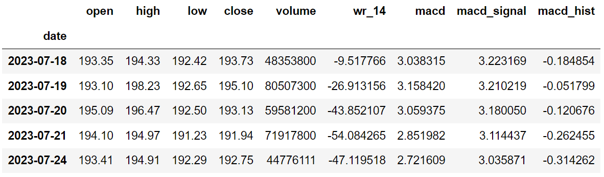
aapl.tail()
Output:
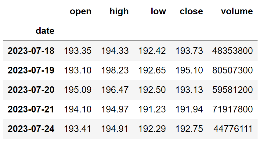
Code Explanation: We initiated by creating a function named ‘get_historical_data’ which takes the stock’s symbol (‘symbol’) and the starting date of historical data (‘start_date’) as inputs. Inside this function, we defined the API key and URL and stored them in respective variables. We then retrieved historical data in JSON format using the ‘get’ function and stored it in the ‘raw_df’ variable. After cleaning and formatting the raw JSON data, we returned it as a well-structured Pandas dataframe. Finally, we called the function to fetch Apple’s historical data from the start of 2010, saving it in the ‘aapl’ variable for further use.
Step-3: Williams %R Calculation
Moving on to the next step, our objective is to compute the Williams %R values according to the formula we previously covered. Let’s proceed with this calculation.
Python Implementation:
# WILLIAMS %R CALCULATION

def get_wr(high, low, close, lookback):
    highh = high.rolling(lookback).max()
    lowl = low.rolling(lookback).min()
    wr = -100 * ((highh - close) / (highh - lowl))
    return wr

aapl['wr_14'] = get_wr(aapl['high'], aapl['low'], aapl['close'], 14)
aapl.tail()
Output:
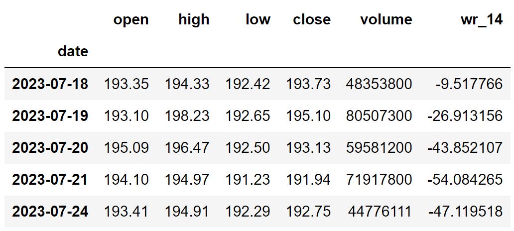
Code Explanation: In this step, we are set to compute the Williams %R values through the implementation of a function labeled ‘get_wr’. This function takes several parameters including the high price data (‘high’), low price data (‘low’), closing price data (‘close’), and the specified lookback period (‘period’).
Here’s a breakdown of the function’s inner workings:
- Determining Highest High and Lowest Low: Within the function, we initially use the ‘rolling’ and ‘max’ functions from the Pandas package to identify the highest high over the designated lookback period. The result is stored in the ‘highh’ variable. Similarly, we utilize the ‘rolling’ and ‘min’ functions to ascertain the lowest low over the same period and store it in the ‘lowl’ variable.
- Calculating Williams %R: With the highest high and lowest low values obtained, we proceed to apply the formula discussed earlier to compute the Williams %R values. These calculated values are stored in the ‘wr’ variable.
- Returning and Calling the Function: Finally, we return the calculated Williams %R values and then call the ‘get_wr’ function itself. This results in the storage of Apple’s Williams %R readings with a lookback period of 14.
Through this process, we successfully calculate the Williams %R values, laying the groundwork for subsequent analysis and strategy development.
Step-4: MACD Calculation
In this particular stage, our focus is directed towards the computation of all the integral components constituting the MACD indicator. These components will be derived from the historical data we’ve extracted for Apple’s stock.
# MACD CALCULATION

def get_macd(price, slow, fast, smooth):
    exp1 = price.ewm(span = fast, adjust = False).mean()
    exp2 = price.ewm(span = slow, adjust = False).mean()
    macd = pd.DataFrame(exp1 - exp2).rename(columns = {'close':'macd'})
    signal = pd.DataFrame(macd.ewm(span = smooth, adjust = False).mean()).rename(columns = {'macd':'signal'})
    hist = pd.DataFrame(macd['macd'] - signal['signal']).rename(columns = {0:'hist'})
    return macd, signal, hist

aapl['macd'] = get_macd(aapl['close'], 26, 12, 9)[0]
aapl['macd_signal'] = get_macd(aapl['close'], 26, 12, 9)[1]
aapl['macd_hist'] = get_macd(aapl['close'], 26, 12, 9)[2]
aapl = aapl.dropna()
aapl.tail()
Output:
Code Explanation: In this step, our task is to calculate the various components that constitute the MACD indicator. Let’s delve into the process of doing so:
We begin by creating a function named ‘get_macd’. This function accepts the stock’s price data (‘prices’), the length of the slow Exponential Moving Average (EMA) (‘slow’), the length of the fast EMA (‘fast’), and the specified period for the Signal line (‘smooth’).
Here’s a breakdown of the function’s functionality:
- Calculating EMAs: Within the function, we first compute the fast and slow length EMAs using the ‘ewm’ (exponential weighted moving average) function provided by Pandas. The computed values are stored in ’ema1′ and ’ema2′ variables respectively.
- MACD Line Calculation: The next step involves calculating the values for the MACD line by subtracting the slow EMA values from the fast EMA values. These values are stored as a Pandas dataframe in the ‘macd’ variable.
- Signal Line Calculation: We create a variable named ‘signal’ to store the values of the Signal line. These values are derived by computing the EMA of the MACD line values (‘macd’) for the specified number of periods.
- Histogram Calculation: The final computation involves determining the Histogram values. This is accomplished by subtracting the MACD line values (‘macd’) from the Signal line values (‘signal’), and these results are stored in the ‘hist’ variable.
- Returning Calculated Values: Ultimately, we return all the calculated values – the MACD line values, Signal line values, and Histogram values.
By implementing these calculations, we successfully derive the MACD components for Apple’s stock data. This sets the stage for the subsequent stages of our analysis and strategy formulation.
Step-5: Creating the Trading Strategy:
In this stage, we are poised to put into practice the trading strategy that combines both the Williams %R and Moving Average Convergence/Divergence (MACD) indicators. This strategy will be implemented using Python programming. Let’s proceed with the implementation of this combined trading strategy.
Python Implementation:
# TRADING STRATEGY

def implement_wr_macd_strategy(prices, wr, macd, macd_signal):
    buy_price = []
    sell_price = []
    wr_macd_signal = []
    signal = 0

    for i in range(len(wr)):
        if wr[i-1] > -50 and wr[i] < -50 and macd[i] > macd_signal[i]:
            if signal != 1:
                buy_price.append(prices[i])
                sell_price.append(np.nan)
                signal = 1
                wr_macd_signal.append(signal)
            else:
                buy_price.append(np.nan)
                sell_price.append(np.nan)
                wr_macd_signal.append(0)

        elif wr[i-1] < -50 and wr[i] > -50 and macd[i] < macd_signal[i]:
            if signal != -1:
                buy_price.append(np.nan)
                sell_price.append(prices[i])
                signal = -1
                wr_macd_signal.append(signal)
            else:
                buy_price.append(np.nan)
                sell_price.append(np.nan)
                wr_macd_signal.append(0)

        else:
            buy_price.append(np.nan)
            sell_price.append(np.nan)
            wr_macd_signal.append(0)

    return buy_price, sell_price, wr_macd_signal

buy_price, sell_price, wr_macd_signal = implement_wr_macd_strategy(aapl['close'], aapl['wr_14'], aapl['macd'], aapl['macd_signal'])
Code Explanation: In this step, we’re putting our trading strategy into action by implementing it through Python code. Here’s how it’s done:
We commence by defining a function named ‘wr_macd_strategy’. This function takes several parameters: stock prices (‘prices’), Williams %R readings (‘wr’), MACD line readings (‘macd’), and Signal line readings (‘macd_signal’).
Here’s a concise description of the function’s logic:
- Initializing Lists: Within the function, we create three empty lists: ‘buy_price’, ‘sell_price’, and ‘wr_macd_signal’. These lists will be used to store values as we execute the trading strategy.
- Implementing Strategy: Using a for-loop, we proceed to implement the trading strategy. Within the loop, we evaluate specific conditions. If these conditions are met, the corresponding values are appended to the previously created lists. Specifically, if the criteria for buying the stock are satisfied, the buying price is appended to the ‘buy_price’ list, and a signal value of 1 is appended to ‘wr_macd_signal’. Similarly, if the criteria for selling the stock are met, the selling price is added to the ‘sell_price’ list, and a signal value of -1 is appended to ‘wr_macd_signal’.
- Returning Appended Lists: At the end of the loop, we return the lists containing the appended values – ‘buy_price’, ‘sell_price’, and ‘wr_macd_signal’.
By executing this function, we successfully apply our trading strategy based on the combined readings of Williams %R and MACD indicators. This lays the foundation for subsequent analysis and evaluation of our strategy’s performance.
Step-6: Creating our Position
Moving forward, our focus shifts to the creation of a list that essentially serves as an indicator of whether we are holding the stock or not. This list will consist of values: 1 indicating that we hold the stock and 0 indicating that we don’t. Let’s proceed with the creation of this list.
Python Implementation:
# POSITION
position = []
for i in range(len(wr_macd_signal)):
if wr_macd_signal[i] > 1:
position.append(0)
else:
position.append(1)
for i in range(len(aapl['close'])):
if wr_macd_signal[i] == 1:
position[i] = 1
elif wr_macd_signal[i] == -1:
position[i] = 0
else:
position[i] = position[i-1]
close_price = aapl['close']
wr = aapl['wr_14']
macd_line = aapl['macd']
signal_line = aapl['macd_signal']
wr_macd_signal = pd.DataFrame(wr_macd_signal).rename(columns = {0:'wr_macd_signal'}).set_index(aapl.index)
position = pd.DataFrame(position).rename(columns = {0:'wr_macd_position'}).set_index(aapl.index)
frames = [close_price, wr, macd_line, signal_line, wr_macd_signal, position]
strategy = pd.concat(frames, join = 'inner', axis = 1)
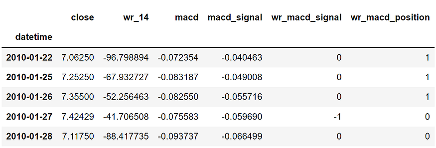
strategy.head()
Output:
Code Explanation: In this stage, our objective is to establish a list that indicates whether we currently hold the stock or not. Here’s how we accomplish this task:
- Initializing the List: To start, we create an empty list called ‘position’.
- Creating Position Values: We employ two for-loops for generating values in the ‘position’ list, aligning its length with that of the ‘signal’ list. The first loop serves to prepare the list with values that match the length of the ‘signal’ list.
- Generating Position Indicators: In the second loop, we iterate through the ‘signal’ list’s values. Depending on the specific conditions met, we append values to the ‘position’ list. A value of 1 is appended if we hold the stock, while a value of 0 is appended if we have sold or do not own the stock.
- Data Manipulation: Towards the end, we perform some data manipulation tasks to combine the various lists that have been created into a single dataframe.
As evident from the output displayed, the ‘position’ in the stock remains consistent at 1 across the first three rows. However, the position shifts to 0 as we sell the stock upon the trading signal indicating a buy signal (-1). The position will maintain a value of -1 until any changes in the trading signal occur.
Now that we have established this essential list, we are prepared to move forward with implementing backtesting procedures.
Step-7: Backtesting
Backtesting involves testing the effectiveness of a trading strategy using historical market data. In our case, we will be using this process to evaluate how well our combined Williams %R and MACD trading strategy performs when applied to historical data of Apple’s stock.
Python Implementation:
# BACKTESTING

aapl_ret = pd.DataFrame(np.diff(aapl['close'])).rename(columns = {0:'returns'})
wr_macd_strategy_ret = []

for i in range(len(aapl_ret)):
    try:
        returns = aapl_ret['returns'][i] * strategy['wr_macd_position'][i]
        wr_macd_strategy_ret.append(returns)
    except:
        pass

wr_macd_strategy_ret_df = pd.DataFrame(wr_macd_strategy_ret).rename(columns = {0:'wr_macd_returns'})

investment_value = 100000
wr_macd_investment_ret = []

for i in range(len(wr_macd_strategy_ret_df['wr_macd_returns'])):
    number_of_stocks = floor(investment_value / aapl['close'][i])
    returns = number_of_stocks * wr_macd_strategy_ret_df['wr_macd_returns'][i]
    wr_macd_investment_ret.append(returns)

wr_macd_investment_ret_df = pd.DataFrame(wr_macd_investment_ret).rename(columns = {0:'investment_returns'})
total_investment_ret = round(sum(wr_macd_investment_ret_df['investment_returns']), 2)
profit_percentage = floor((total_investment_ret / investment_value) * 100)
print(cl('Profit gained from the W%R MACD strategy by investing $100k in AAPL : {}'.format(total_investment_ret), attrs = ['bold']))
print(cl('Profit percentage of the W%R MACD strategy : {}%'.format(profit_percentage), attrs = ['bold']))
Output:
Profit gained from the W%R MACD strategy by investing $100k in AAPL : 239805.45
Profit percentage of the W%R MACD strategy : 239%
Code Explanation: Initially, we compute the returns for Apple stock using the ‘diff’ function from NumPy, and these returns are stored as a dataframe in the ‘aapl_ret’ variable. Subsequently, we employ a for-loop to iterate over the ‘aapl_ret’ values, calculating the returns obtained from our trading strategy. These calculated returns are then appended to the ‘wr_macd_strategy_ret’ list. To structure the data neatly, we convert this list into a dataframe named ‘wr_macd_strategy_ret_df’.
The subsequent step involves backtesting. This entails testing our strategy’s effectiveness by investing $100,000 into it. The investment value is stored in the ‘investment_value’ variable. We then compute the quantity of Apple stocks that can be purchased using this investment amount. To ensure that we deal with integers, we use the ‘floor’ function from the Math package, which eliminates decimals. Notably, this function differs from the ’round’ function.
Through a for-loop, we ascertain the investment returns, followed by certain data manipulations. Ultimately, we print the total return derived from investing $100,000 in our trading strategy. The result reveals an approximate profit of $240,000 over around thirteen-and-a-half years, yielding a profit percentage of 239%. This performance is impressive! Subsequently, we proceed to compare our returns with those of the SPY ETF, an Exchange-Traded Fund designed to track the S&P 500 stock market index.
Step-8: SPY ETF Comparison
While this step is not mandatory, it is strongly advised as it provides valuable insights into how our trading strategy fares against a benchmark, specifically the SPY ETF. In this stage, we will retrieve data for the SPY ETF using the ‘get_historical_data’ function we established earlier. We will then proceed to compare the returns obtained from the SPY ETF with the returns generated by our trading strategy applied to Apple’s stock data.
Python Implementation:
# SPY ETF COMPARISON

def get_benchmark(start_date, investment_value):
    spy = get_historical_data('SPY', start_date)['close']
    benchmark = pd.DataFrame(np.diff(spy)).rename(columns = {0:'benchmark_returns'})

    investment_value = investment_value
    benchmark_investment_ret = []

    for i in range(len(benchmark['benchmark_returns'])):
        number_of_stocks = floor(investment_value/spy[i])
        returns = number_of_stocks*benchmark['benchmark_returns'][i]
        benchmark_investment_ret.append(returns)

    benchmark_investment_ret_df = pd.DataFrame(benchmark_investment_ret).rename(columns = {0:'investment_returns'})
    return benchmark_investment_ret_df

benchmark = get_benchmark('2010-01-01', 100000)
investment_value = 100000
total_benchmark_investment_ret = round(sum(benchmark['investment_returns']), 2)
benchmark_profit_percentage = floor((total_benchmark_investment_ret/investment_value)*100)
print(cl('Benchmark profit by investing $100k : {}'.format(total_benchmark_investment_ret), attrs = ['bold']))
print(cl('Benchmark Profit percentage : {}%'.format(benchmark_profit_percentage), attrs = ['bold']))
print(cl('W%R MACD Strategy profit is {}% higher than the Benchmark Profit'.format(profit_percentage - benchmark_profit_percentage), attrs = ['bold']))
Output:
Benchmark profit by investing $100k : 159541.51
Benchmark Profit percentage : 159%
W%R MACD Strategy profit is 80% higher than the Benchmark Profit
Code Explanation: The code employed in this phase closely resembles the one employed in the preceding backtesting step. However, in this instance, the investment pertains to the SPY ETF, and no trading strategies are implemented. Upon examining the output, it becomes evident that our trading strategy has surpassed the performance of the SPY ETF by an impressive 80%. This outcome is indeed commendable!
Final Thoughts!
After an extensive journey through both theoretical and programming aspects, we have successfully delved into the intricacies of Williams %R and Moving Average Convergence/Divergence indicators. By combining these indicators using Python, we’ve constructed a trading strategy that not only makes sense but also delivers profits.
However, there’s always room for improvement. One area to explore is the creation of more intricate trading strategies. Relying on just two indicators doesn’t guarantee success in the volatile market. It’s advisable to devise fresh, innovative, and unconventional strategies, testing them across various stocks, timeframes, and scenarios.
Another crucial consideration is strategy evaluation. Evaluating a trading strategy goes beyond simply observing profits or returns. It involves a thorough assessment of multiple factors. While we’ve directly focused on profits in this article, strategy evaluation provides a deeper understanding with practical and realistic insights.
Lastly, but significantly, is risk management. Risk management is a cornerstone of trading, a concept that should be rigorously implemented in any trading system. While we haven’t covered this aspect here, its importance cannot be understated. It’s imperative to ensure proper risk management measures are in place before implementing any strategy in the real market.
It’s worth noting that each of these concepts merits its own in-depth exploration, extending well beyond the scope of a single article section. With that, you’ve reached the conclusion of this article. I hope you’ve gained new and valuable insights from this exploration.