Stock price prediction is a programmatically tedious task, especially when done with exquisite detail. From choosing the right models to building and evaluating them, the whole process demands patience and meticulous execution. However, with the emergence of powerful AI tools like ChatGPT, we might have a shot at predicting the market with ease.
In this article, we will first obtain the time series data of the stock we are willing to predict using the EODHD End-of-day API, then, we will feed this data into the program generated by ChatGPT. All the processes including data preparation, building the model, making predictions, and model evaluation will be taken care of by ChatGPT. Without further ado, let’s dive into the article!
Quick jump:
Project Outline
After a series of conversations with ChatGPT regarding the models that can be used for stock price prediction, the methodology to be followed, etc., it gave me an overwhelming number of choices to choose from. But I decided to keep it simple and wanted to follow the most sought-after method of predicting stock prices which is through using an LSTM model.
I then asked ChatGPT for help drafting an outline for an extensive LSTM Python project for predicting stock prices and this is what it generated:
1. Obtaining data
2. Linear Regression
3. A basic LSTM model
4. Improving the LSTM model
5. Hyperparameter Tuning
This was not the initial outline generated by the bot, but after conversing for a while, it came up with this, which I think is pretty straightforward and easy to grasp. The entire article will follow this outline and apart from the first section of obtaining data, all the other sections will be solely driven by ChatGPT alone.
1. Obtaining Data using EODHD
To build a successful ML model which can predict with a higher level of accuracy, data of quality and reliability must be preferred over anything else. This is where EODHD comes into play. EOD Historical Data (EODHD) is a reliable provider of financial APIs covering a huge variety of market data ranging from historical data to economic and financial news data.
For this project, we’ll be predicting Microsoft’s stock prices for which we need its time series data for a long period. Thus, I went with EODHD’s end-of-day or historical data API. I used the following code to extract Microsoft’s historical data from 2010 to the present:
def get_historical_data(symbol, start, end):
    api_key = 'YOUR API KEY'
    api_response = requests.get(f'https://eodhistoricaldata.com/api/eod/{symbol}?api_token={api_key}&fmt=json&from={start}&to={end}').json()
    df = pd.DataFrame(api_response).drop('close', axis = 1)
    df.columns = ['Date', 'Open', 'High', 'Low', 'Close', 'Volume']
    df.Date = pd.to_datetime(df.Date)
    return df

df = get_historical_data('MSFT', '2010-01-01', '2023-07-23')
df.to_csv('msft.csv')

df.tail()
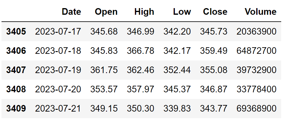
There isn’t anything complicated with this code. For the smooth working of the code, make sure to replace “YOUR API KEY” with your secret EODHD API key which you can obtain after creating an account with them. We are saving the extracted data so that it can be easily imported and fed into the upcoming prediction program rather than making API calls every single time. One thing which I would like to add is that though the API has a data coverage of 30+ years, I’ve decided to keep it 13 as it’s more than enough for our program. This is the final dataframe:
2. Linear Regression
Instead of directly jumping into building an LSTM model, I wanted to take things slowly with ChatGPT to get a glimpse of the results generated by the code given by the bot. So I asked it to write me a Python program to build a basic Linear Regression model using Scikit Learn for the purpose of predicting stock prices. It initially gave me the steps to be followed for building the regression model and then wrote this sample code:
import pandas as pd
import numpy as np
from sklearn.linear_model import LinearRegression
from sklearn.model_selection import train_test_split
from sklearn.preprocessing import StandardScaler
from sklearn.metrics import r2_score, mean_squared_error
import matplotlib.pyplot as plt

# Get the stock data
df = pd.read_csv('msft.csv').dropna()
df = df.set_index('Date')

# Add a column for the target variable
df['Price'] = df['Close']

# Define the features and target variable
features = ['Open', 'High', 'Low', 'Volume']
target = 'Price'

# Split the data into training and testing sets
train_size = 0.8
train_data = df[:int(train_size * len(df))]
test_data = df[int(train_size * len(df)):]

# Normalize the data
scaler = StandardScaler()
train_data[features] = scaler.fit_transform(train_data[features])
test_data[features] = scaler.transform(test_data[features])

# Train the model
model = LinearRegression()
model.fit(train_data[features], train_data[target])

# Make predictions on the test data
predictions = model.predict(test_data[features])

# Compute the R^2 score and RMSE
r2 = r2_score(test_data[target], predictions)
rmse = np.sqrt(mean_squared_error(test_data[target], predictions))

print(f'R^2 score: {r2:.4f}')
print(f'RMSE: {rmse:.4f}')

# Plot the predicted and actual values
plt.plot(test_data[target].values, label='Actual')
plt.plot(predictions, label='Predicted')
plt.legend()
plt.show()
This code is surprisingly well-formatted and incorporates all the conventional procedures. One of the best things about this code are the comments which are included in each and every process, making it easier to understand what is going on. It also gave a short brief about the code to explain the whole process. Now, these are the results of the code:
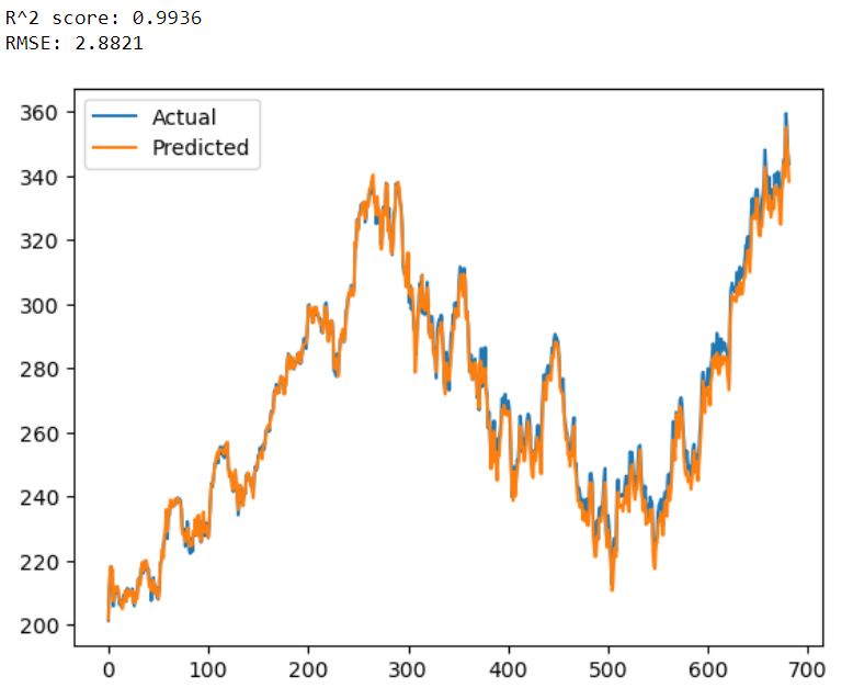
One small thing I would do with this code is to play with the model parameters to ascertain the most ideal model for our case but this is a topic for another day because the focus here is to get an understanding of ChatGPT’s code and its results.
3. A basic LSTM model
Now it’s time to up the game and ask ChatGPT to generate a Python program to build an LSTM model for predicting stock prices. But before moving on, here is a short description of LSTM: Long Short-Term Memory (LSTM) is a sophisticated neural network and a powerful tool for analyzing sequential data. It selectively stores or forgets information to understand complex sequences of data. This makes it ideal for tasks like speech recognition, natural language processing, and analyzing time-series data. Here’s the code generated by ChatGPT to build a predictive LSTM model:
import numpy as np
import pandas as pd
import matplotlib.pyplot as plt
from sklearn.metrics import *
from sklearn.preprocessing import MinMaxScaler
from tensorflow.keras.models import Sequential
from tensorflow.keras.layers import LSTM, Dense, Dropout

# Load the stock price data
df = pd.read_csv('msft.csv').dropna()
df = df.set_index('Date')

# Preprocess the data
scaler = MinMaxScaler()
df_scaled = scaler.fit_transform(df['Close'].values.reshape(-1, 1))

# Define the training and testing data
train_size = int(len(df_scaled) * 0.8)
train_data = df_scaled[:train_size, :]
test_data = df_scaled[train_size:, :]

# Define the function to create a sliding window dataset
def create_dataset(dataset, time_steps=1):
    X_data, y_data = [], []
    for i in range(len(dataset)-time_steps-1):
        X_data.append(dataset[i:(i+time_steps), 0])
        y_data.append(dataset[i + time_steps, 0])
    return np.array(X_data), np.array(y_data)

# Define the time steps and create the sliding window dataset
time_steps = 60
X_train, y_train = create_dataset(train_data, time_steps)
X_test, y_test = create_dataset(test_data, time_steps)

# Reshape the data for LSTM input
X_train = np.reshape(X_train, (X_train.shape[0], X_train.shape[1], 1))
X_test = np.reshape(X_test, (X_test.shape[0], X_test.shape[1], 1))

# Define the LSTM model architecture
model = Sequential()
model.add(LSTM(units=64, return_sequences=True, input_shape=(X_train.shape[1], 1)))
model.add(Dropout(0.2))
model.add(LSTM(units=64, return_sequences=True))
model.add(Dropout(0.2))
model.add(LSTM(units=64, return_sequences=False))
model.add(Dropout(0.2))
model.add(Dense(units=1))

# Compile the model
model.compile(optimizer='adam', loss='mean_squared_error')

# Train the model
model.fit(X_train, y_train, epochs=50, batch_size=64, validation_data=(X_test, y_test), verbose=1)

# Make predictions
y_pred = model.predict(X_test)

# Inverse transform the predicted and actual values
y_pred = scaler.inverse_transform(y_pred)
y_test = y_test.reshape(y_pred.shape[0], 1)
y_test = scaler.inverse_transform(y_test)

# Evaluate the model
mse = mean_squared_error(y_test, y_pred)
msle = mean_squared_log_error(y_test, y_pred)
mae = mean_absolute_error(y_test, y_pred)
r2 = r2_score(y_test, y_pred)

print('MSE: ', mse)
print('MSLE: ', msle)
print('MAE: ', mae)
print('R-squared: ', r2)

# Plot the predicted vs actual values
plt.figure(figsize=(10, 6))
plt.style.use('fivethirtyeight')
plt.plot(y_test, label='Actual', linewidth = 3, alpha = 0.4)
plt.plot(y_pred, label='Predicted', linewidth = 1.5)
plt.xlabel('Days')
plt.ylabel('Stock Price')
plt.title('LSTM: Actual vs Predicted')
plt.legend()
plt.show()
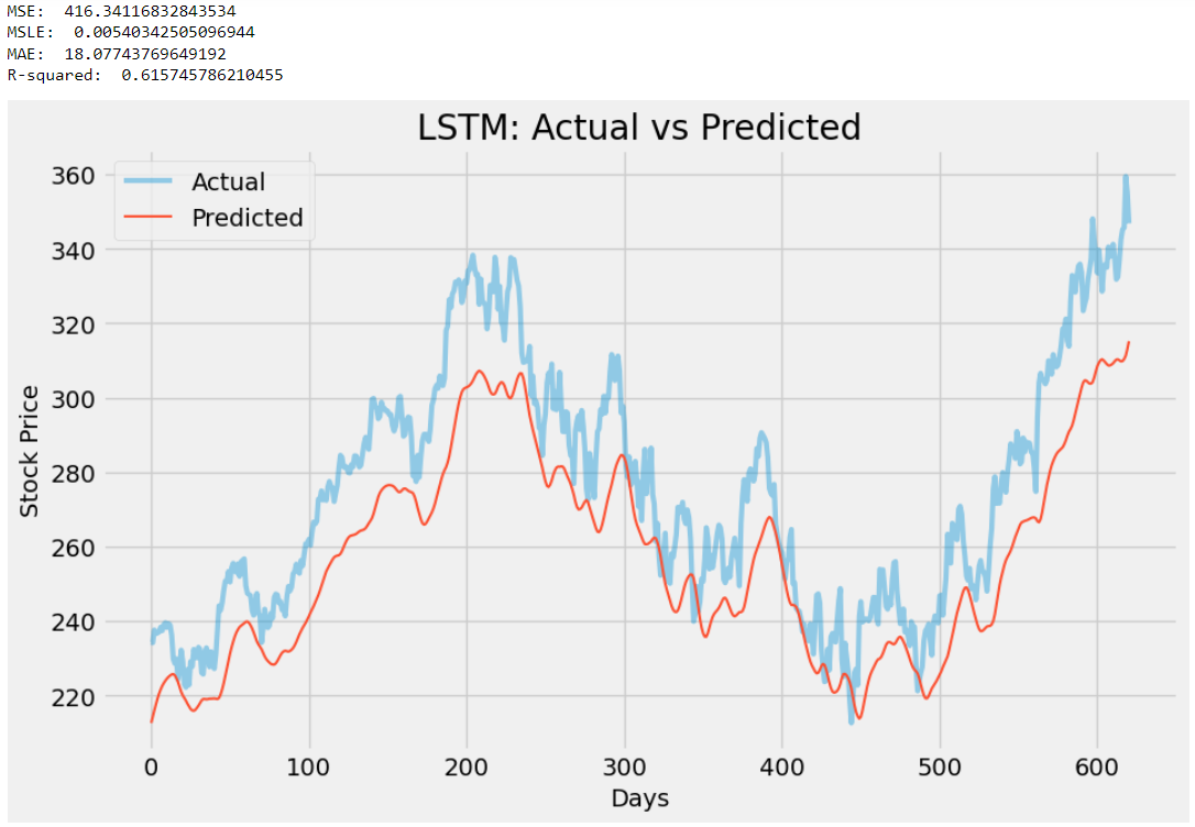
This code is very simple yet amazingly clear and again well-formatted with wonderful comments for each step of the code. ChatGPT followed a very straightforward way of using TensorFlow to build an LSTM model which I think is perfectly fine because that’s what I asked for and I love the evaluation process that comes along with a graph. I did customize the plot by adding some additional parameters to beautify it but other than that, I didn’t touch a single line of code. Here’s the result:
4. Improving the LSTM model
The LSTM model which we just built and used for prediction is very simplistic in nature and can be improved in various aspects. So I asked ChatGPT to give me some suggestions to improve the code for a better LSTM model and here’s what it got to say about it:
- Increase the number of LSTM layers: One way to improve the model’s performance is to add more LSTM layers to the model. This can help the model capture more complex patterns in the data.
- Increase the number of neurons in each layer: Another way to improve the model’s performance is to increase the number of neurons in each LSTM layer. This can help the model learn more complex relationships between the input features and the target variable.
- Adjust the learning rate: The learning rate determines how much the model adjusts its weights in response to the error between the predicted and actual values. A small learning rate can slow down the training process, while a large learning rate can cause the model to overshoot the optimal weights. Tuning the learning rate can improve the model’s performance.
- Add dropout layers: Dropout layers can be added to the model to prevent overfitting. This technique randomly drops out some neurons during training, which can help the model generalize better to new data.
- Try different activation functions: The choice of activation function can affect the model’s ability to learn complex relationships in the data. Experimenting with different activation functions such as tanh, relu, and sigmoid can help improve the model’s performance.
- Use more data: Increasing the amount of data used to train the model can improve its performance. This can be achieved by either increasing the number of years of historical data or using additional features such as news sentiment data or technical indicators.
- Use a different loss function: The choice of the loss function can also affect the model’s performance. Using a loss function that is more appropriate for time series data, such as mean squared logarithmic error (MSLE), can help improve the model’s accuracy.
This is awesome! It just gave us a complete guideline to be followed in order to improve an AI model, specifically LSTM in our case. I then asked ChatGPT to include all these suggestions in the previous code and it returned me this updated version:
import numpy as np
import pandas as pd
import matplotlib.pyplot as plt
from sklearn.metrics import *
from sklearn.preprocessing import MinMaxScaler
from tensorflow.keras.models import Sequential
from tensorflow.keras.layers import LSTM, Dense, Dropout
from tensorflow.keras.callbacks import EarlyStopping

# Obtain stock data for Microsoft
df = pd.read_csv('msft.csv').dropna()

# Extract the closing prices
close_prices = df[["Date", "Close"]].copy()
close_prices.columns = ["ds", "y"]
close_prices.set_index("ds", inplace=True)

# Normalize the data
scaler = MinMaxScaler(feature_range=(0, 1))
close_prices_scaled = scaler.fit_transform(close_prices)

# Create training and testing data
train_size = int(len(close_prices) * 0.8)
train_data = close_prices_scaled[:train_size]
test_data = close_prices_scaled[train_size:]

# Define the number of time steps to look back
look_back = 60

# Create training and testing data for the LSTM model
def create_data(data):
    X, Y = [], []
    for i in range(look_back, len(data)):
        X.append(data[i - look_back : i, 0])
        Y.append(data[i, 0])
    X, Y = np.array(X), np.array(Y)
    X = np.reshape(X, (X.shape[0], X.shape[1], 1))
    return X, Y

X_train, Y_train = create_data(train_data)
X_test, Y_test = create_data(test_data)

# Define the LSTM model
model = Sequential()

model.add(LSTM(units=64, return_sequences=True, input_shape=(X_train.shape[1], 1)))
model.add(Dropout(0.2))

model.add(LSTM(units=128, return_sequences=True))
model.add(Dropout(0.2))

model.add(LSTM(units=64))
model.add(Dropout(0.2))

model.add(Dense(units=1))

# Compile the model
model.compile(optimizer="adam", loss="mean_squared_error")

# Define the early stopping criteria
early_stop = EarlyStopping(monitor="val_loss", patience=10)

# Fit the model to the training data
history = model.fit(X_train, Y_train, epochs=100, batch_size=32, validation_data=(X_test, Y_test), callbacks=[early_stop])

# Make predictions on the test data
y_pred = model.predict(X_test)

# Inverse the scaling of the data
y_pred = scaler.inverse_transform(y_pred)
Y_test = scaler.inverse_transform([Y_test])

# Evaluate the model
mse = mean_squared_error(Y_test[0], y_pred)
msle = mean_squared_log_error(Y_test[0], y_pred)
mae = mean_absolute_error(Y_test[0], y_pred)
r2 = r2_score(Y_test[0], y_pred)

print('MSE: ', mse)
print('MSLE: ', msle)
print('MAE: ', mae)
print('R-squared: ', r2)

# Plot the predicted vs actual values
plt.figure(figsize=(10, 6))
plt.style.use('fivethirtyeight')
plt.plot(Y_test.flatten(), label="Actual", linewidth = 3, alpha = 0.4)
plt.plot(y_pred.flatten(), label="Predicted", linewidth = 1.5)
plt.title("MSFT Stock Price Prediction")
plt.xlabel("Days")
plt.ylabel("Stock Price")
plt.legend()
plt.show()
This code is a sort of extended version of the previous code with all those little changes suggested by ChatGPT. According to ChatGPT: It increases the number of LSTM layers, increases the number of neurons in each layer, adds dropout layers, and adjusts the learning rate. It also uses more data by training on the entire historical data and uses a different loss function, mean squared logarithmic error (MSLE), which is more appropriate for time series data.
In my opinion, there aren’t any significant changes to the code, but that is acceptable because it is not necessary to bring in a great number of modifications to improve an existing model. Here is a side-by-side comparison of the results of both models (left: previous model, right: improved model):

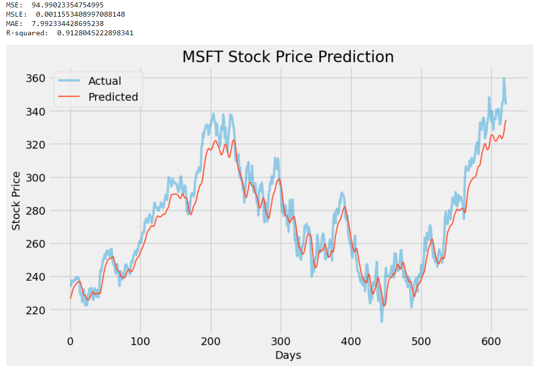
By observing the results, we can conclude that there are some great improvements made in the performance of the LSTM model. The R2 score of the new model has increased from 0.61 to 0.91 (yowza!) indicating higher prediction accuracy, and the MSE, MSLE, and MAE scores are all significantly reduced making them even more closer to zero which is again, a good sign of a better model. Henceforth, ChatGPT really did a great job in improving our model.
5. Hyperparameter Tuning
No AI & ML project is complete without hyperparameter tuning. Here’s a little background about hyperparameter tuning: The process which involves adjusting the settings of a machine learning model to improve its performance is called hyperparameter tuning. These settings, known as hyperparameters, are set before training the model and include parameters such as learning rate, number of layers and neurons, etc. The primary objective of fine-tuning these settings is to boost the model’s accuracy in predictions. Here’s the code ChatGPT generated when asked to perform hyperparameter tuning on the previously generated model:
import numpy as np
import pandas as pd
from sklearn.preprocessing import MinMaxScaler
from tensorflow.keras.models import Sequential
from tensorflow.keras.layers import Dense, LSTM, Dropout
from tensorflow.keras.optimizers import Adam
from tensorflow.keras.wrappers.scikit_learn import KerasRegressor
from sklearn.model_selection import GridSearchCV, TimeSeriesSplit

# Download the data
df = pd.read_csv('msft.csv').dropna()
df = df.set_index('Date')

# Scale the data
scaler = MinMaxScaler()
scaled_data = scaler.fit_transform(df['Close'].values.reshape(-1, 1))

# Define the training and test sets
train_size = int(len(scaled_data) * 0.8)
train_data = scaled_data[:train_size]
test_data = scaled_data[train_size:]

# Define the function to create the LSTM model
def create_model(neurons=50, layers=2, dropout=0.2, learning_rate=0.001):
    model = Sequential()
    for i in range(layers):
        model.add(LSTM(units=neurons, return_sequences=True, input_shape=(train_data.shape[1], 1)))
        model.add(Dropout(dropout))
    model.add(LSTM(units=neurons))
    model.add(Dropout(dropout))
    model.add(Dense(units=1))
    optimizer = Adam(learning_rate=learning_rate)
    model.compile(optimizer=optimizer, loss='mean_squared_error')
    return model

# Define the parameter grid for hyperparameter tuning
param_grid = {
    'neurons': [50, 100, 200],
    'layers': [2, 3],
    'dropout': [0.2, 0.3],
    'learning_rate': [0.001, 0.01]
}

# Define the time series split for cross-validation
tscv = TimeSeriesSplit(n_splits=3)

# Create the KerasRegressor for hyperparameter tuning
model = KerasRegressor(build_fn=create_model, epochs=50, batch_size=32, verbose=0)

# Perform the hyperparameter tuning
grid = GridSearchCV(estimator=model, param_grid=param_grid, cv=tscv, scoring='neg_mean_squared_error', n_jobs=-1)
grid_result = grid.fit(train_data, train_data)

# Print the best parameters and score
print("Best parameters: ", grid_result.best_params_)
print("Best score: ", np.sqrt(-grid_result.best_score_))

# Use the best model to make predictions on the test data
best_model = grid_result.best_estimator_.model
predictions = best_model.predict(test_data.reshape(-1, 1))
predictions = scaler.inverse_transform(predictions)

# Plot the predictions and actual values
import matplotlib.pyplot as plt

# Plot the predicted vs actual values
plt.figure(figsize=(10, 6))
plt.style.use('fivethirtyeight')
plt.plot(pd.to_datetime(df.index[train_size:]), df['Close'][train_size:], label='Actual', linewidth = 3, alpha = 0.4)
plt.plot(pd.to_datetime(df.index[train_size:]), predictions, label='Predicted', linewidth = 1.5)
plt.title(f"MSFT Stock Price Prediction")
plt.xlabel("Date")
plt.ylabel("Stock Price")
plt.legend()
plt.show()
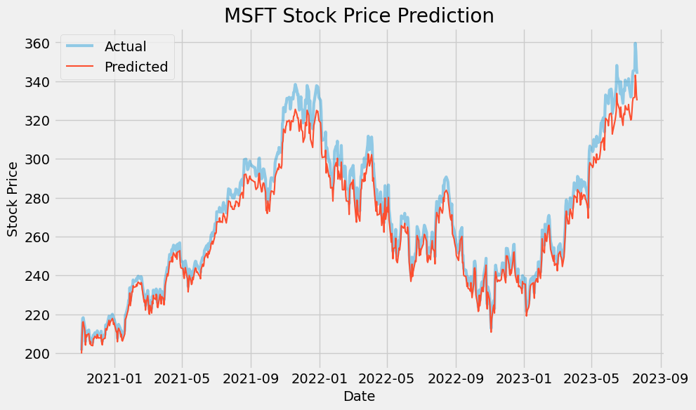
Just like all the other programs generated before, this code also follows a clean structure, neatly written comments, and a pretty well-known procedure of hyperparameter tuning which is to define a “param_grid” and pass the grid to the “GridSearchCV” function to perform a Grid Search and ascertain the best model parameters. These are the best parameters according to the hyperparameter tuning process by ChatGPT:
Best parameters:  {'dropout': 0.2, 'layers': 2, 'learning_rate': 0.001, 'neurons': 100}
Best score:  0.0047933462470134474
ChatGPT did not stop there and went further to use the best parameters to build a model and make predictions. This graph is the final result of the model derived from hyperparameter tuning:
Final Thoughts
Although ChatGPT helped us in crafting some amazing code to predict stock prices, the models mostly become obsolete in the real-world market because the prices are entirely driven by personal emotions and sentiments, which are factors that cannot be quantified or measured using code generated by a bot.
That doesn’t mean the work we have done so far is absolute garbage, it is rather a starting point for the actual analysis. Getting an idea of the price movement through these AI models gives us some direction or a layout of the approach that should be followed for analyzing the stock. So, predictive analytics should only be viewed as a secondary tool when it comes to making investment decisions rather than trusting it blindfolded.
A huge shoutout to EODHD for creating such an amazing warehouse of financial APIs. I really love their platform because the data they provide is incredibly accurate which ultimately helped in boosting the model performance in a substantial way. I highly recommend checking out their platform and many may find it greatly useful for their future projects and endeavors.
With that being said, you’ve reached the end of the article. Hope you learned something new.

