

We all learn early on that taking on more risk can lead to bigger rewards. Basically, this means that the more a stock price swings, the greater its potential gain. Does that sound familiar? But here’s an interesting twist: many traders talk about something called the low-volatility anomaly. This idea suggests that stocks with less price fluctuation can sometimes give you even better returns when you consider the risk involved, compared to their more volatile peers.
Here, I’ll put this theory to the test by attempting to identify the anomaly. The approach will involve calculating rolling volatility from daily stock prices, ranking stocks monthly, and building an equal-weighted portfolio of the least and most volatile stocks, using data from the EODHD suite of APIs.
Let’s write some Python
Let’s set up our imports and parameters
import os
from tqdm import tqdm
import pandas as pd
import numpy as np
import requests
import requests_cache
import matplotlib.pyplot as plt

api_token = os.environ.get('EODHD_API_TOKEN')

START_DATE = '2015-01-01'
UNIVERSE_INDEX = 'GSPC.INDX'  # EODHD index code for S&P 500
N_VOL = 10
ROLLING_WINDOW = 22  # ~1 month trading days
As you can see, we’ll use the EODHD API suite to retrieve the last 10 years of prices to date. For our backtesting universe, we’ll obtain the SP500 stocks. EODHD provides an endpoint that enumerates the current constituents of the S&P 500 as well as their historical memberships, including the respective start and end dates during which each stock was part of this prestigious index.
url = 'https://eodhd.com/api/mp/unicornbay/spglobal/comp/{}'.format(UNIVERSE_INDEX)
r = requests.get(url, params={'api_token': api_token, 'fmt': 'json'})
data = r.json()
df_symbols = pd.DataFrame(data['HistoricalTickerComponents']).T.reset_index()
df_symbols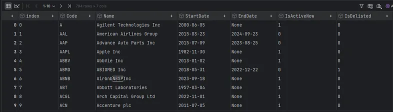
That will give us a total of 794 stocks that were part of the SP500 over the years. We’ll also add the sector using the relevant EODHD fundamentals endpoint, so we can get the sector in our analysis later.
def fetch_fundamentals(code, exchange='US'):
    ticker = f"{code}.{exchange}"
    url = f'https://eodhd.com/api/fundamentals/{ticker}'
    try:
        resp = requests.get(url, params={'api_token': api_token, 'fmt': 'json'}, timeout=30)
        if resp.status_code != 200:
            return None, None
        js = resp.json() if resp.content else {}
        general = js.get('General', {}) if isinstance(js, dict) else {}
        highlights = js.get('Highlights', {}) if isinstance(js, dict) else {}
        sector = general.get('Sector')
        return sector
    except Exception:
        return None


records = []
for code in tqdm(df_symbols['Code'].astype(str).unique(), desc='Fetching fundamentals'):
    sector = fetch_fundamentals(code, 'US')
    records.append({'Code': code, 'Sector': sector})

fund_df = pd.DataFrame(records)
df_symbols = df_symbols.drop(columns=[c for c in ['Sector'] if c in df_symbols.columns]) \
    .merge(fund_df, on='Code', how='left')

symbols = (df_symbols['Code'].astype(str) + '.US').tolist()
Now, let’s dive into the main analysis. First, I’ll create a dataframe called all_adj_close to work with the adjusted closing prices from the last 10 years, giving us a solid foundation for our insights.
# Function to fetch data for a single ticker
def fetch_stock_data(ticker, start_date):
url = f'https://eodhd.com/api/eod/{ticker}'
query = {
'api_token': api_token,
'fmt': 'json',
'from': start_date,
}
url = f'https://eodhd.com/api/eod/{ticker}'
query = {
'api_token': api_token,
'fmt': 'json',
'from': start_date,
}
response = requests.get(url, params=query)
if response.status_code != 200:
print(f"Error fetching data for {ticker}: {response.status_code}")
print(response.text)
return None
try:
data = response.json()
df = pd.DataFrame(data)
df['date'] = pd.to_datetime(df['date'])
df.set_index('date', inplace=True)
df.sort_index(inplace=True) # Ensure data is sorted by date
return df
except Exception as e:
return None
# Create an empty DataFrame to store adjusted close prices
all_adj_close = pd.DataFrame()
# Prepare SP500 membership intervals per ticker (from df_symbols)
tmp_members = df_symbols[['Code', 'StartDate', 'EndDate']].copy()
tmp_members['StartDate'] = pd.to_datetime(tmp_members['StartDate'], errors='coerce')
tmp_members['EndDate'] = pd.to_datetime(tmp_members['EndDate'], errors='coerce') # NaT means still active
membership_ranges = {}
for _, row in tmp_members.iterrows():
code = str(row['Code'])
start = row['StartDate']
end = row['EndDate'] # can be NaT
if pd.isna(start):
continue
membership_ranges.setdefault(code, []).append((start, end))
# Fetch data for each ticker and add to the DataFrame
for ticker in tqdm(symbols):
stock_data = fetch_stock_data(ticker, START_DATE)
if stock_data is not None:
# Extract ticker symbol without exchange suffix for column name
symbol = ticker.split('.')[0]
all_adj_close[symbol] = stock_data['adjusted_close']
# Create SP500 membership indicator per date for this ticker
dates = stock_data.index
in_sp500 = pd.Series(False, index=dates)
for (start, end) in membership_ranges.get(symbol, []):
if pd.isna(end):
mask = dates >= start
else:
mask = (dates >= start) & (dates <= end)
if mask.any():
in_sp500.loc[mask] = True
all_adj_close[symbol + "_IN_SP500"] = in_sp500.astype(int) # 1 if in SP500, 0 otherwise
rets = stock_data['adjusted_close'].pct_change()
all_adj_close[symbol + "_PCT_CHANGE"] = rets
vol = rets.rolling(ROLLING_WINDOW).std()
all_adj_close[symbol + "_VOL"] = vol
else:
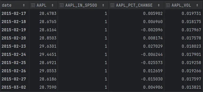
passLet me explain what we are doing here:
- For each symbol, we’ll gather the daily closing prices at the end of the day. Our dataframe will have one column for each symbol, named after it. For example, AAPL.
- Additionally, since we’re there, we’ll also calculate the daily percentage change (e.g. AAPL_PCT_CHANGE), which helps us determine the rolling volatility over 22 days (roughly a month), referred to as AAPL_VOL in our example.
- Additionally, we’ll have a field for each ticker ending in _IN_SP500, which shows whether the specific stock was included in the S&P 500 on that day.
Next, we need to create two columns for the highest and lowest volatility tickers, as comma-separated strings, at the start of each month. These will only include stocks that were part of the S&P 500 on the first day.
Since our investment portfolio doesn’t need changes daily, we’ll rebalance it once a month. This way, we can stay focused and ensure everything stays on track.
dates_first = all_adj_close.index[all_adj_close.index.day == 1].unique()

records = []
for d in dates_first:
    # Identify volatility columns where the equivalent _IN_SP500 is 1 on date d
    vol_cols = [
        c for c in all_adj_close.columns
        if c.endswith('_VOL') and all_adj_close.at[d, c[:-4] + '_IN_SP500'] == 1
    ]

    s = all_adj_close.loc[d, vol_cols].dropna()
    if s.empty:
        continue

    # Highest and lowest volatility tickers for the date
    highest = s.sort_values(ascending=False).head(N_VOL).index
    lowest = s.sort_values(ascending=True).head(N_VOL).index

    # Strip the _VOL suffix and join with commas
    highest_str = ",".join([col[:-4] for col in highest])  # remove '_VOL'
    lowest_str = ",".join([col[:-4] for col in lowest])

    records.append({
        'DATE': d,
        'HIGHEST_VOL_TICKERS': highest_str,
        'LOWEST_VOL_TICKERS': lowest_str
    })

monthly_vol_tickers = pd.DataFrame.from_records(records).set_index('DATE').sort_index()
monthly_vol_tickers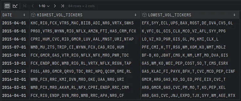
Here’s a dataframe with one row for each month. I’ll add this information to the original dataframe that includes all the prices by month.
mt = monthly_vol_tickers.copy()
mt['MONTH'] = mt.index.to_period('M')

top_map = mt.groupby('MONTH')['HIGHEST_VOL_TICKERS'].last().to_dict()
low_map = mt.groupby('MONTH')['LOWEST_VOL_TICKERS'].last().to_dict()

# Map each date in all_adj_close to its month and fill columns for the entire month
periods = all_adj_close.index.to_period('M')
all_adj_close['HIGHEST_VOL_TICKERS'] = periods.map(top_map)
all_adj_close['LOWEST_VOL_TICKERS'] = periods.map(low_map)
The next step is to calculate the daily percentage change of the stocks we are invested in, as well as the equity curve. Note that:
- For the highest and lowest stocks, I’m using the average percentage change to calculate returns and the equity curve, as we’re assuming equal investment in each stock.
- I’ll also use the S&P 500 index as a reference, but with a small tweak. Instead of relying on the index itself, which is weighted by each stock’s market capitalisation, I’ll calculate the average of the percentage change and equity values for all the symbols in the S&P 500 on that day. This way, we can make a fairer comparison, like comparing apples with apples.
# Prepare symbol to column mappings
_PCT_SUFFIX = '_PCT_CHANGE'
_IN_SUFFIX = '_IN_SP500'

pct_cols = [c for c in all_adj_close.columns if c.endswith(_PCT_SUFFIX)]
symbols_from_pct = [c[:-len(_PCT_SUFFIX)] for c in pct_cols]

pct_col_by_symbol = {sym: f'{sym}{_PCT_SUFFIX}' for sym in symbols_from_pct}
in_col_by_symbol = {sym: f'{sym}{_IN_SUFFIX}' for sym in symbols_from_pct}


def avg_for_list(row, list_col_name):
    syms_str = row.get(list_col_name, np.nan)
    if not isinstance(syms_str, str) or not syms_str:
        return np.nan
    syms = [s.strip() for s in syms_str.split(',') if s.strip()]
    cols = [pct_col_by_symbol[s] for s in syms if s in pct_col_by_symbol]
    if not cols:
        return np.nan
    return row[cols].mean(skipna=True)


def avg_for_in_sp500(row):
    syms_in = [s for s in symbols_from_pct if in_col_by_symbol[s] in row.index and row[in_col_by_symbol[s]] == 1]
    cols = [pct_col_by_symbol[s] for s in syms_in if pct_col_by_symbol[s] in row.index]
    if not cols:
        return np.nan
    return row[cols].mean(skipna=True)


# Compute new columns
all_adj_close['AVG_PCT_CHANGE_HIGHEST_VOL'] = all_adj_close.apply(lambda r: avg_for_list(r, 'HIGHEST_VOL_TICKERS'),
                                                                  axis=1)
all_adj_close['AVG_PCT_CHANGE_LOWEST_VOL'] = all_adj_close.apply(lambda r: avg_for_list(r, 'LOWEST_VOL_TICKERS'),
                                                                 axis=1)
all_adj_close['AVG_PCT_CHANGE_IN_SP500'] = all_adj_close.apply(avg_for_in_sp500, axis=1)

all_adj_close[['AVG_PCT_CHANGE_HIGHEST_VOL', 'AVG_PCT_CHANGE_LOWEST_VOL', 'AVG_PCT_CHANGE_IN_SP500']]

cols = ['AVG_PCT_CHANGE_HIGHEST_VOL', 'AVG_PCT_CHANGE_LOWEST_VOL', 'AVG_PCT_CHANGE_IN_SP500']
rets = all_adj_close[cols].fillna(0.0)
equity_curves = (1.0 + rets).cumprod()
Now let’s plot…
plt.figure(figsize=(12, 6))
for c in equity_curves.columns:
    plt.plot(equity_curves.index, equity_curves[c], label=c)
plt.title('Equity Curves')
plt.xlabel('Date')
plt.ylabel('Equity (Start=1.0)')
plt.legend()
plt.grid(True)
plt.tight_layout()
plt.show()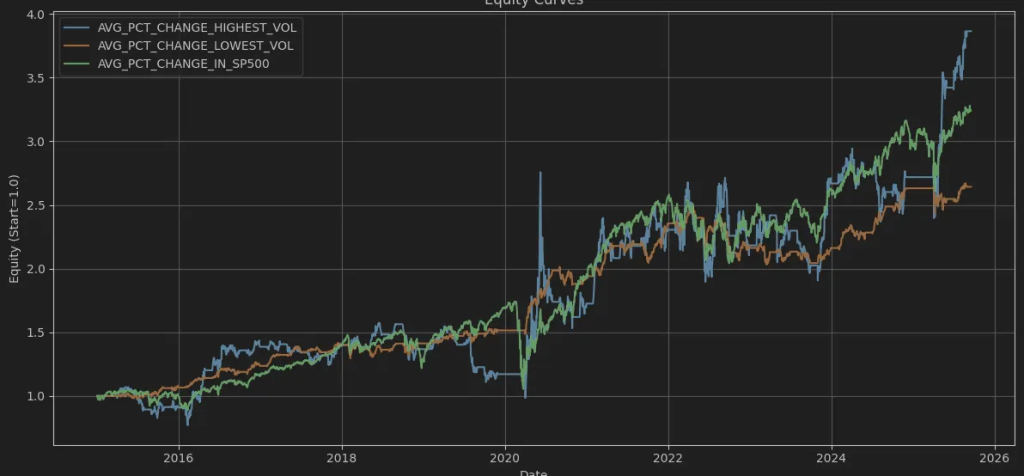
As you can see, the anomaly we’re discussing can’t be identified and doesn’t appear in the long run. What the theory states is also shown in the graph:
Higher returns are linked to higher volatility, while lower returns are associated with lower volatility. The S&P 500, with equally weighted returns, falls somewhere in between.
So, let’s see what happens if we apply the same concept to specific sectors. The only thing you need to do is add the following code right after you finish and run the code again.
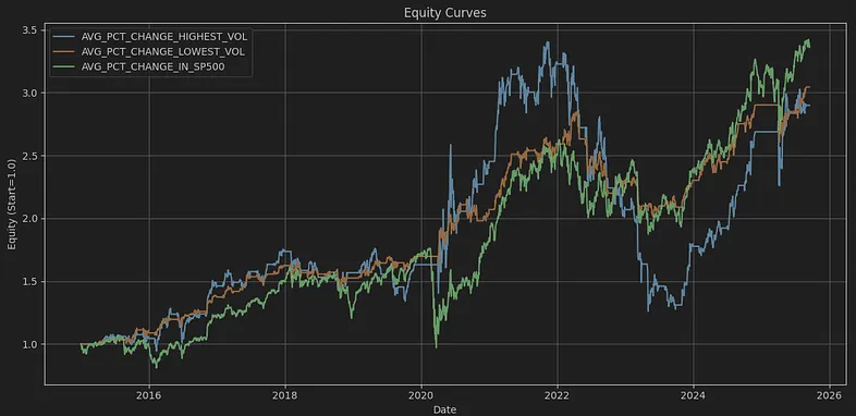
df_symbols = df_symbols[df_symbols['Sector'].isin(['Technology'])].copy()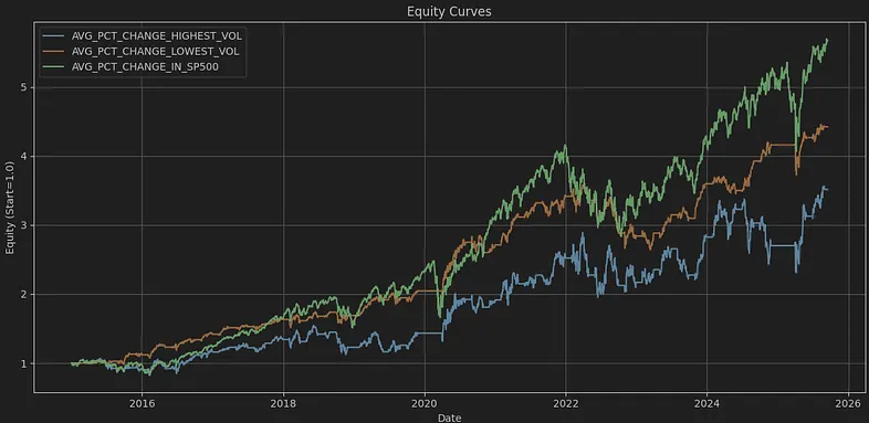
That’s really interesting! In the tech world, while SP_500 stocks usually do quite well, it’s so fascinating to see that the stocks with the lowest volatility often perform better than those with higher volatility. I believe this might be because technology stock fundamentals change so rapidly, making a stock swing from high to low volatility in just a few months. It seems like sticking to the middle range might be the safest and smartest bet here ;).
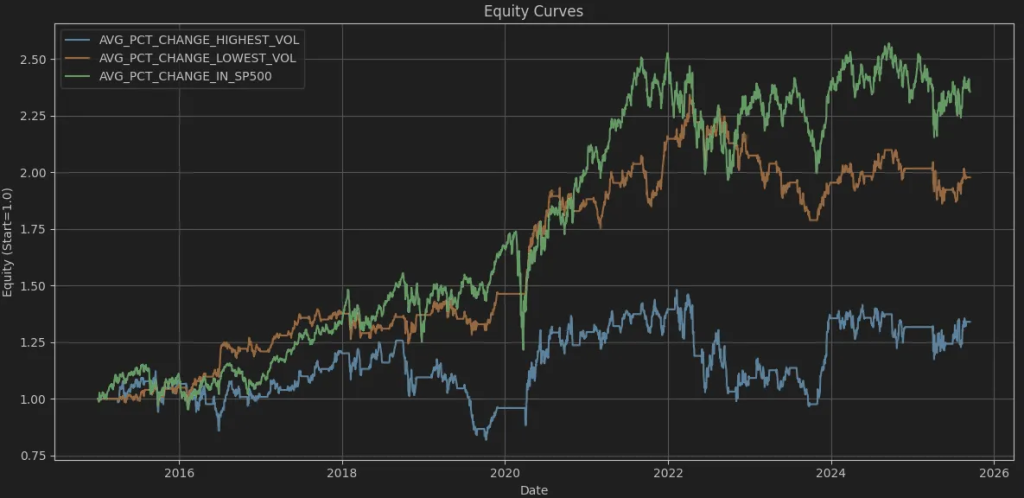
Let’s see what happens with Financial Services.
Nevertheless, the SP_500 outperforms all of them in this case. The interesting part is that, with Financial Services, it is very clear that there are huge returns and drawdowns for the high-volatility stocks, while the low-volatility ones tend to move more slowly at the same time. It appears that Financial Services stocks tend to move more smoothly, making the low-volatility stocks more attractive.
What about Healthcare?
That’s also interesting. High-volatility healthcare stocks don’t seem to follow the typical higher-risk, higher-reward rule. Since healthcare is a defensive sector with steady demand, the stocks still experience significant peaks and troughs due to regulatory decisions, drug trial results, and similar factors. Personally, I avoid volatile healthcare stocks.
Conclusions
- Over 10 years, S&P 500 stocks showed higher returns for high-volatility portfolios and low-volatility anomaly was not detected.
- Within Technology, low-volatility stocks performed better than high-volatility stocks, suggesting sector-specific effects on the anomaly.
- Financial Services: high-volatility stocks had significant swings but fell behind the equally-weighted S&P 500; low-volatility stocks maintained steady movement.
- Healthcare stocks with high volatility failed to outperform, probably due to regulatory and drug trial factors that led to unpredictable returns.
What I took away from this analysis for myself is that the low-volatility anomaly isn’t a universal phenomenon. Sector dynamics and fundamentals have a significant impact on risk-return relationships.
Thank you for reading. I hope you enjoyed it!