How to Trade using the Fibonacci Time Zones with Python

Last year I wrote a popular article on the Fibonacci Sequence and how it’s used in trading (it can be found here). The article introduced two topics, namely Fibonacci Retracement Levels and Fibonacci Extension Levels. There are two additional topics called Fibonacci Time Zones and Fibonacci Arcs and Fans that are interesting as well. This article will cover Fibonacci Time Zones using data from the EODHD APIs Python library.

Register & Get Data

What is the Fibonacci Sequence?

The Fibonacci Sequence is a series of numbers where each number is the sum of the two preceding numbers, usually starting from 0. The sequence is as follows: 0, 1, 1, 2, 3, 5, 8, 13, 21, 34, etc.

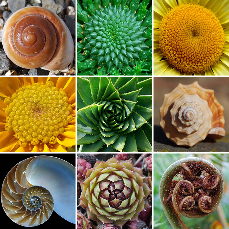
The Fibonacci Sequence is remarkably prevalent in nature, often signifying an underlying order in biological structures and phenomena. Here are just a few examples:

1. The spiral pattern of leaves around a stem of plants.
2. Number of petals on a variety of flowers E.g., 3, 5, 21, 34, 55, 89, etc.
3. Tree branches forming every 5th row of bark.
4. The spirals on and inside fruit and vegetables.
5. Animals that have spiral shells.
6. Some animals reproduce in numbers that follow the Fibonacci sequence.
7. The DNA molecule, the fundamental building block of life, measures 34 angstroms long by 21 angstroms wide for each full cycle of its double helix spiral, both Fibonacci numbers.

These occurrences are often related to the concept of the “golden ratio” (approximately 1.618), a closely related concept where the ratio of two consecutive Fibonacci numbers approximates the golden ratio, especially as the sequence progresses. The “golden ratio” was covered in my previous article when calculating the Fibonacci Retracement and Extension levels.

How is the Fibonacci Sequence used in Trading?

It’s not just nature where the Fibonacci Sequence and the “golden ratio” has been identified. There is a strong correlation with financial markets and it’s often used as a tool in technical analysis.

It’s important to understand that, like all technical analysis tools, Fibonacci methods are not a guarantee of future market movements. It is used to gauge potential future events based on historical patterns and should always be used in conjunction with other analysis methods and sound risk management strategies.

Let’s look at an example…

For this tutorial I’m going to retrieve Apple’s (AAPL) hourly data using the EODHD APIs Python library. If you don’t already have a subscription with EODHD APIs, you will need to obtain an API Token.

You will want to install (or upgrade) the following Python libraries for this tutorial.

$ python3 -m pip install eodhd pandas mplfinance matplotlib -U

Create yourself a config.py with your API key.

API_KEY="<YOUR_KEY>"

We then will want to instantiate the API.

api = APIClient(cfg.API_KEY)

Register & Get Data

Create our first function that will retrieve our OHLC (Open, High, Low, Close) data for Apple (AAPL) using the EODHD API. The Pandas dataframe returned via the API is a time series with the timestamp reflected as the index. I actually want to use this as a column for plotting the data, so I will copy the “datetime” index to a “datetime” column.

def get_ohlc_data():
    df = api.get_historical_data("AAPL", "1h")
    df["datetime"] = df.index
    return df

We then need a function that will identify the significant highs and lows. This is done by calculating the rolling minimum and maximum value.

def find_significant_points(ohlc_data, window=10):
    ohlc_data["rolling_max"] = ohlc_data["high"].rolling(window=window).max()
    ohlc_data["rolling_min"] = ohlc_data["low"].rolling(window=window).min()
    significant_highs = ohlc_data[ohlc_data["high"] == ohlc_data["rolling_max"]]
    significant_lows = ohlc_data[ohlc_data["low"] == ohlc_data["rolling_min"]]
    return significant_highs, significant_lows

Once we have our significant highs and lows we want to calculate the Fibonacci Time Zones using the sequence. I have omitted the proceeding 0 and 1, and I have only plotted up to 89. You can adjust this more or less than you need but it’s about right.

def fibonacci_intervals(start_date, num_periods=100):
    fib_sequence = [1, 2, 3, 5, 8, 13, 21, 34, 55, 89]  # etc.
    intervals = [
        start_date + pd.Timedelta(days=x) for x in fib_sequence if x <= num_periods
    ]
    return intervals

The next step is optional but I always like to see the data visually. This function will plot the pricing data, including the significant highs and lows, and potential Fibonacci reversal points.

def plot_fibonacci_with_ohlc(
    ohlc_data, significant_highs, significant_lows, fib_intervals
):
    ohlc_data["date_num"] = mdates.date2num(ohlc_data["datetime"])
    fig, ax = plt.subplots(figsize=(12, 6))

    candlestick_ohlc(
        ax,
        ohlc_data[["date_num", "open", "high", "low", "close"]].values,
        width=0.6,
        colorup="green",
        colordown="red",
    )

    for date in fib_intervals:
        ax.axvline(x=mdates.date2num(date), color="blue", linestyle="--", lw=0.5)

    ax.scatter(
        mdates.date2num(significant_highs["datetime"]),
        significant_highs["high"],
        marker="^",
        color="green",
        label="Significant Highs",
    )
    ax.scatter(
        mdates.date2num(significant_lows["datetime"]),
        significant_lows["low"],
        marker="v",
        color="red",
        label="Significant Lows",
    )

    ax.xaxis_date()
    ax.xaxis.set_major_formatter(mdates.DateFormatter("%Y-%m-%d"))
    plt.xticks(rotation=45)
    plt.xlabel("Date")
    plt.ylabel("Price")
    plt.title("OHLC Data with Fibonacci Timing Intervals")
    plt.legend()
    plt.tight_layout()
    plt.show()

This code will retrieve the OHLC data and calculate the significant highs and lows. I’m printing it to the screen for demonstration purposes.

ohlc_data = get_ohlc_data()
highs, lows = find_significant_points(ohlc_data)

print("Significant Highs:")
print(highs)

print("\nSignificant Lows:")
print(lows)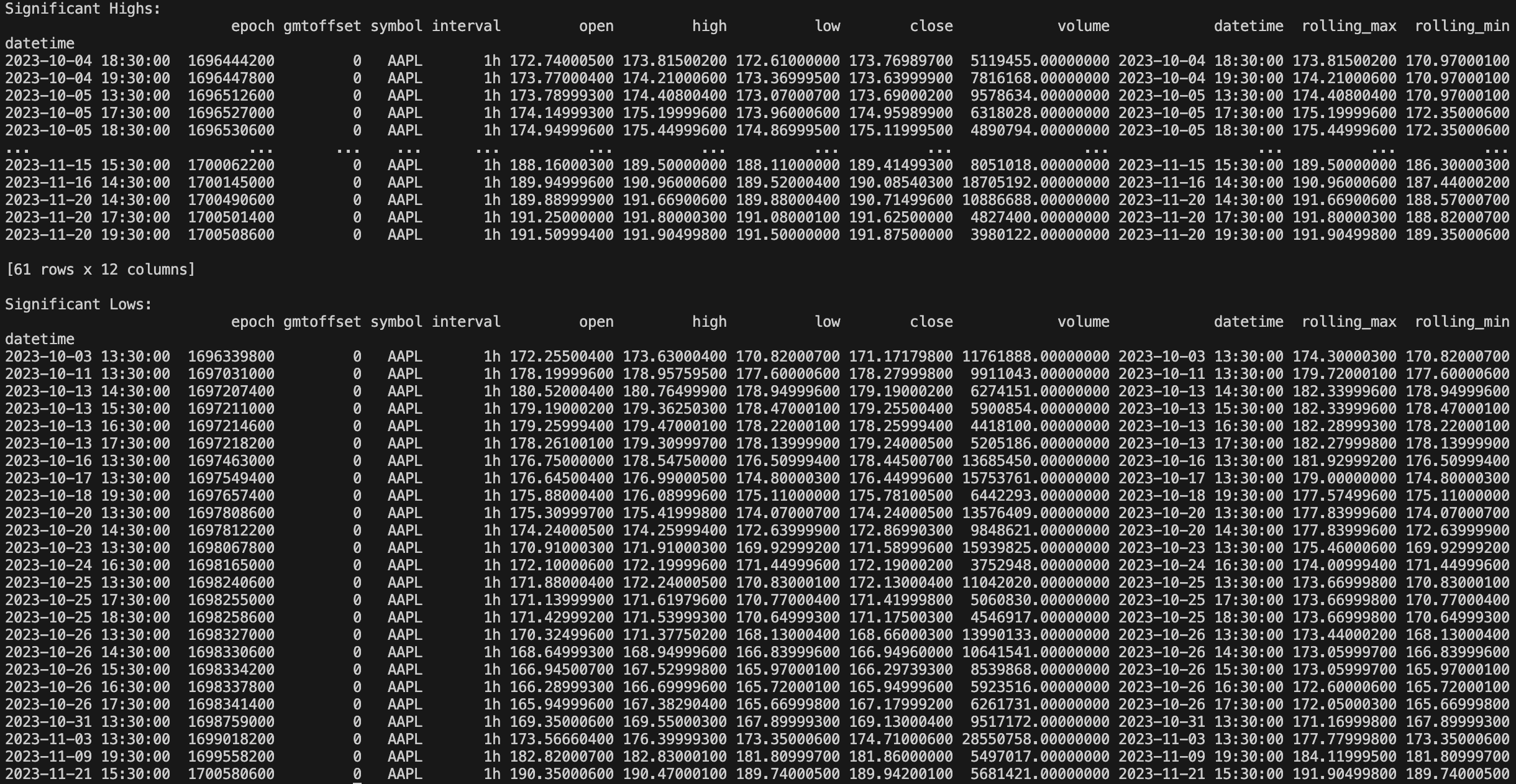

What we will do now is take the first significant high and calculate the Fibonacci timing intervals from there. The 0 reflects the first significant high.

start_date = highs.iloc[0]["datetime"]  # first significant high
fib_intervals = fibonacci_intervals(start_date)

print("Fibonacci Timing Intervals from start date", start_date)
for date in fib_intervals:
    print(date)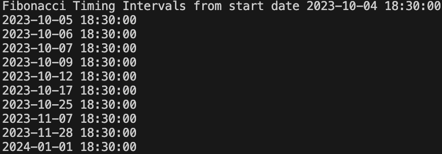

We can now visualise it with Matplotlib like this.

plot_fibonacci_with_ohlc(ohlc_data, highs, lows, fib_intervals)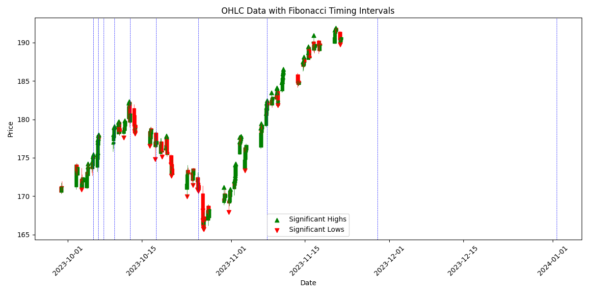

This graph is displaying the Apple hourly candlestick data with a scattergraph overlaid showing the significant highs in green and significant lows in red. It’s also showing the Fibonacci intervals from the first significant high.

Register & Get Data

Conclusion

Using the Fibonacci sequence has been shown to be effective, but it’s not advisable to use it in isolation. Always apply additional technical analysis to strengthen the conclusion of a buy or sell signal.