Each of the indicators Bollinger Bands, Keltner Channel, and Relative Strength Index are unique in nature and powerful when used individually. But what if we try to combine all these three indicators and create one effective trading strategy out of them? The results would be substantial, and we could be able to eradicate one of the most common problems associated with using technical indicators, which is false signals.

That’s exactly what we aim to do today. In this article, we will first build some basic intuitions on the indicators, then we will use Python to build them from scratch, construct a trading strategy out of them, backtest the strategy with real-world historical stock data, and compare the results with those of SPY ETF (an ETF specifically designed to track the movement of the S&P 500 market index).

Quick jump:

1 Bollinger Bands
2 Keltner Channel (KC)
3 Relative Strength Index
4 Trading Strategy
5 Implementation in Python

Bollinger Bands

Before jumping on to explore Bollinger Bands, it is essential to know what a simple moving average (SMA) is. A simple moving average is just the average price of a stock given a specified period of time. Now, Bollinger Bands are trend lines plotted above and below the SMA of the given stock at a specific standard deviation level. To understand Bollinger Bands better, have a look at the following chart that represents the Bollinger Bands of the Apple stock calculated with SMA 20.

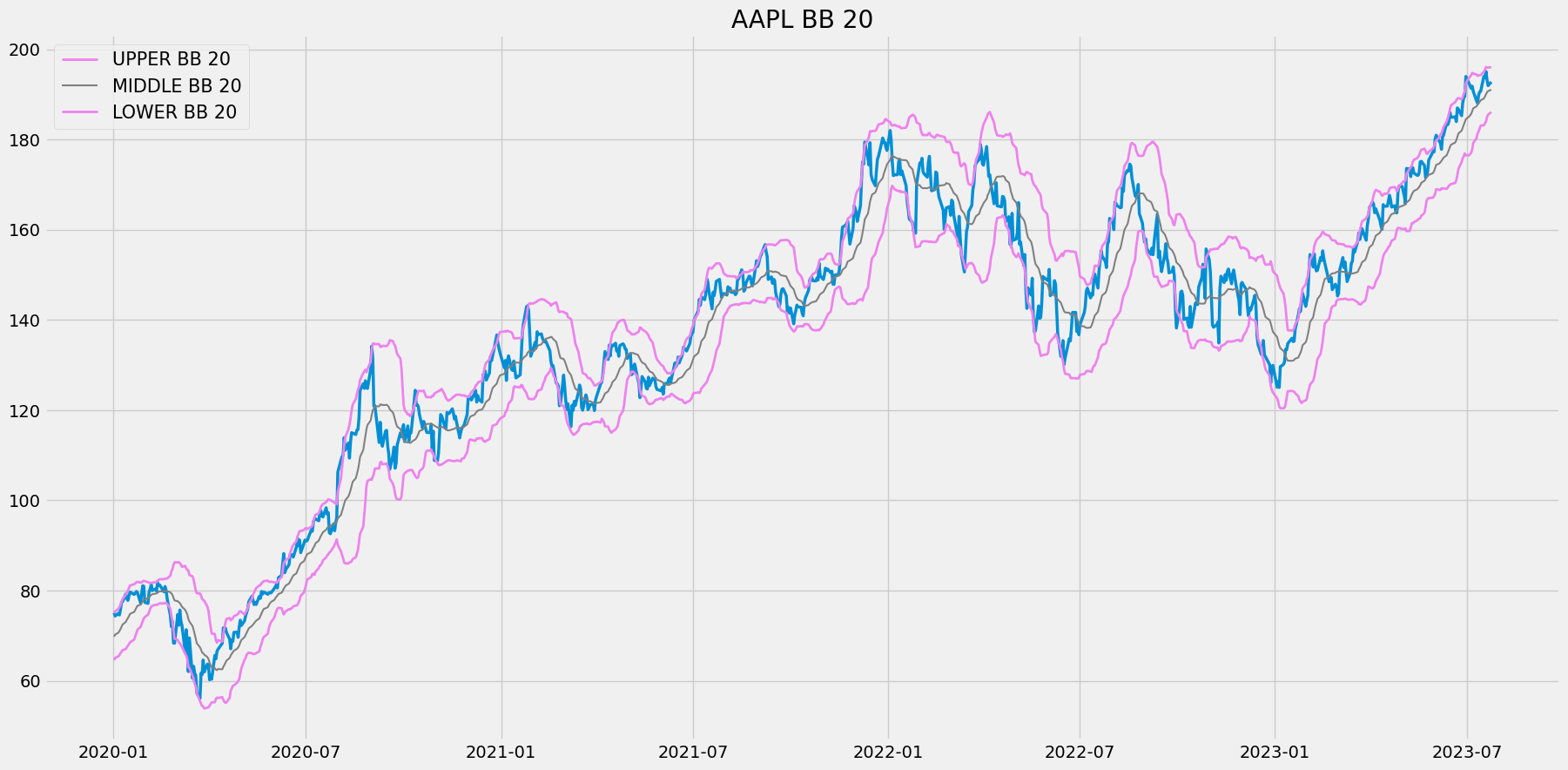
Bollinger Bands are great to observe the volatility of a given stock over a period of time. The volatility of a stock is observed to be lower when the space or distance between the upper and lower band is less. Similarly, when the space or distance between the upper and lower band is more, the stock has a higher level of volatility. While observing the chart, you can observe a trend line named ‘MIDDLE BB 20’ which is the SMA 20 of the Apple stock. The formula to calculate both upper and lowers bands of stock is as follows:

UPPER_BB = STOCK SMA + SMA STANDARD DEVIATION * 2
LOWER_BB = STOCK SMA - SMA STANDARD DEVIATION * 2

Keltner Channel (KC)

First introduced by Chester Keltner, the Keltner Channel is a technical indicator that is often used by traders to identify volatility and the direction of the market. The Keltner Channel is composed of three components: The upper band, the lower band, and the middle line. Now, let’s discuss how each of the components is calculated.

Before diving into the calculation of the Keltner Channel it is essential to know about the three important inputs involved in the calculation. First is the ATR (Average True Range) lookback period, which is the number of periods that are taken into account for the calculation of ATR. Secondly, the Keltner Channel lookback period. This input is more or less similar to the first one but here, we are determining the number of periods that are taken into account for the calculation of the Keltner Channel itself. The final input is the multiplier which is a value determined to multiply with the ATR. The typical values that are taken as inputs are 10 as the ATR lookback period, 20 as the Keltner Channel lookback period, and 2 as the multiplier. Keeping these inputs in mind, let’s calculate the readings of the Keltner Channel’s components.

The first step in calculating the components of the Keltner Channel is determining the ATR values with 10 as the lookback period.

The next step is calculating the middle line of the Keltner Channel. This component is the 20-day Exponential Moving Average of the closing price of the stock. The calculation can be represented as follows:

MIDDLE LINE 20 = EMA 20 [ C.STOCK ]

where,
EMA 20 = 20-day Exponential Moving Average 
C.STOCK = Closing price of the stock

The final step is calculating the upper and lower bands. Let’s start with the upper band. It is calculated by first adding the 20-day Exponential Moving Average of the closing price of the stock by the multiplier (two) and then, multiplied by the 10-day ATR. The lower band calculation is almost similar to that of the upper band but instead of adding, we will be subtracting the 20-day EMA by the multiplier. The calculation of both upper and lower bands can be represented as follows:

UPPER BAND 20 = EMA 20 [ C.STOCK ] + MULTIPLIER * ATR 10
LOWER BAND 20 = EMA 20 [ C.STOCK ] - MULTIPLIER * ATR 10

where,
EMA 20 = 20-day Exponential Moving Average 
C.STOCK = Closing price of the stock
MULTIPLIER = 2
ATR 10 = 10-day Average True Range

That’s the whole process of calculating the components of the Keltner Channel. Now, let’s analyze a chart of the Keltner Channel to build more understanding of the indicator.

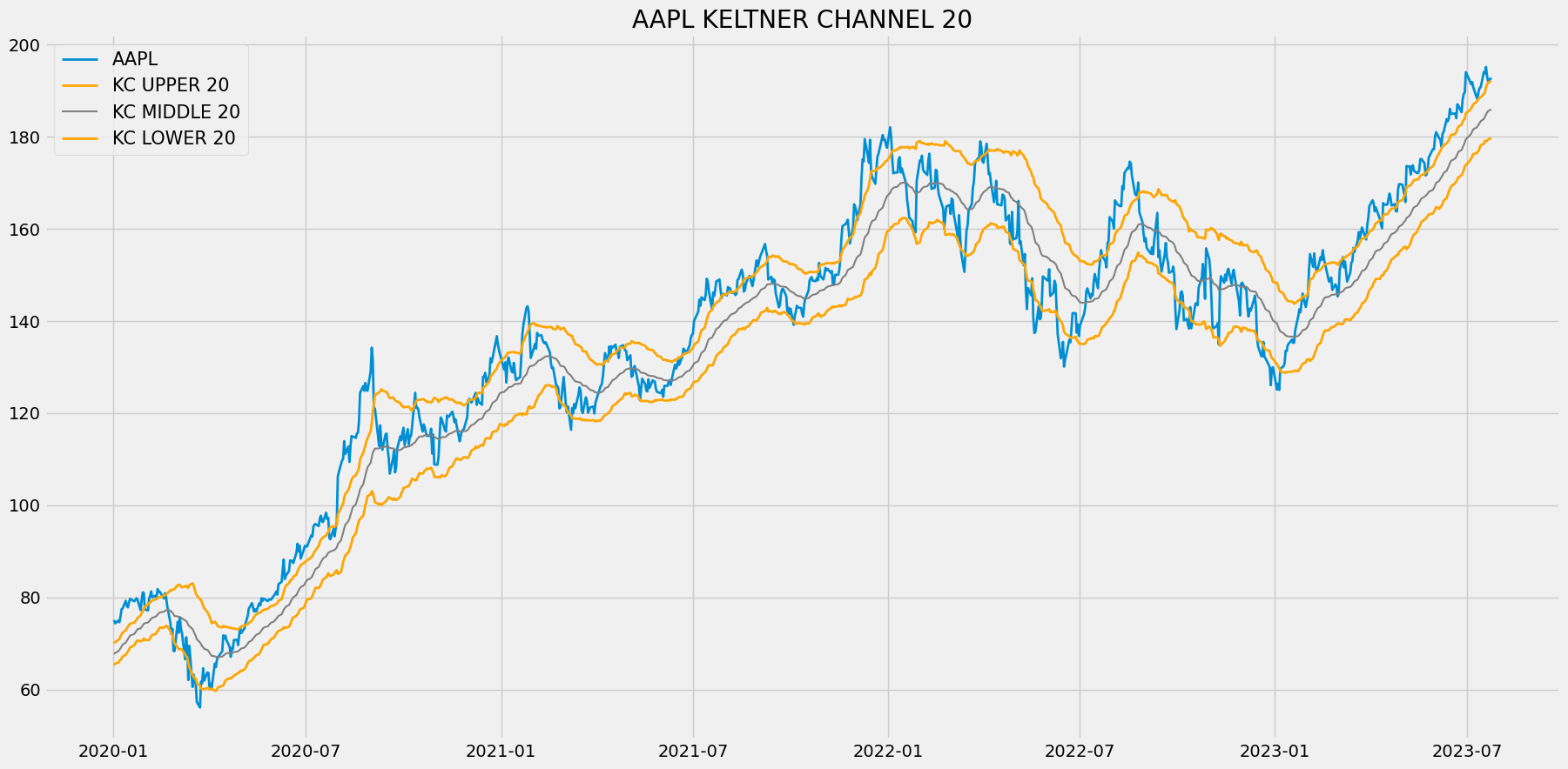
The above chart is a graphical representation of Apple’s 20-day Keltner Chanel. We could notice that two bands are plotted on either side of the closing price line and those are the upper and lower band, and the grey-colored line running in between the two bands is the middle line, or the 20-day EMA. The Keltner Channel can be used in an extensive number of ways but the most popular usages are identifying the market volatility and direction.

The volatility of the market can be determined by the space that exists between the upper and lower band. If the space between the bands is wider, then the market is said to be volatile or showing greater price movements. On the other hand, the market is considered to be in a state of non-volatile or consolidating if the space between the bands is narrow. The other popular usage is identifying the market direction. The market direction can be determined by following the direction of the middle line as well as the upper and lower band.

While looking at the chart of the Keltner Channel, it might resemble the Bollinger Bands. The only difference between these two indicators is the way each of them is calculated. The Bollinger Bands use standard deviation for its calculation, whereas, the Keltner Channel utilizes ATR to calculate its readings.

Relative Strength Index

Before moving on, let’s first gain an understanding of what an oscillator means in the stock trading space. An oscillator is a technical tool that constructs a trend-based indicator whose values are bound between a high and low band. Traders use these bands along with the constructed trend-based indicator to identify the market state and make potential buy and sell trades. Also, oscillators are widely used for short-term trading purposes, but there are no restrictions in using them for long-term investments.

Founded and developed by J. Welles Wilder in 1978, the Relative Strength Index is a momentum oscillator that is used by traders to identify whether the market is in a state of overbought or oversold. Before moving on, let’s explore what overbought and oversold is. A market is considered to be in the state of overbought when an asset is constantly bought by traders, moving it to an extremely bullish trend and bound to consolidate. Similarly, a market is considered to be in the state of oversold when an asset is constantly sold by traders, moving it to a bearish trend and tends to bounce back.

Being an oscillator, the values of RSI are bound between 0 to 100. The traditional way to evaluate a market state using the Relative Strength Index is that an RSI reading of 70 or above reveals a state of overbought, and similarly, an RSI reading of 30 or below represents the market is in the state of oversold. These overbought and oversold can also be tuned concerning which stock or asset you choose. For example, some assets might have constant RSI readings of 80 and 20. So in that case, you can set the overbought and oversold levels to be 80 and 20 respectively. The standard setting of RSI is 14 as the lookback period.

RSI might sound more similar to Stochastic Oscillator in terms of value interpretation, but the way it’s being calculated is quite different. There are three steps involved in the calculation of RSI:

Calculating the Exponential Moving Average (EMA) of the gain and loss of an asset: A word on Exponential Moving Average. EMA is a type of Moving Average (MA) that automatically allocates greater weighting (nothing but importance) to the most recent data point and lesser weighting to data points in the distant past. In this step, we will first calculate the returns of the asset and separate the gains from losses. Using these separated values, the two EMAs for a specified number of periods are calculated.
Calculating the Relative Strength of an asset: The Relative Strength of an asset is determined by dividing the Exponential Moving Average of the gain of an asset from the Exponential Moving Average of the loss of an asset for a specified number of periods. It can be mathematically represented as follows:

RS = GAIN EMA / LOSS EMA

where,
RS = Relative Strength
GAIN EMA = Exponential Moving Average of the gains
LOSS EMA = Exponential Moving Average of the losses

Calculating the RSI values: In this step, we will calculate the RSI itself by making use of the Relative Strength values we calculated in the previous step. To calculate the values of RSI of a given asset for a specified number of periods, there is a formula that we need to follow:

RSI = 100.0 - (100.0 / (1.0 + RS))

where,
RSI = Relative Strength Index
RS = Relative Strength

Now let’s analyze a chart of RSI plotted along with Apple’s historical stock data to gain a strong understanding of the indicator.

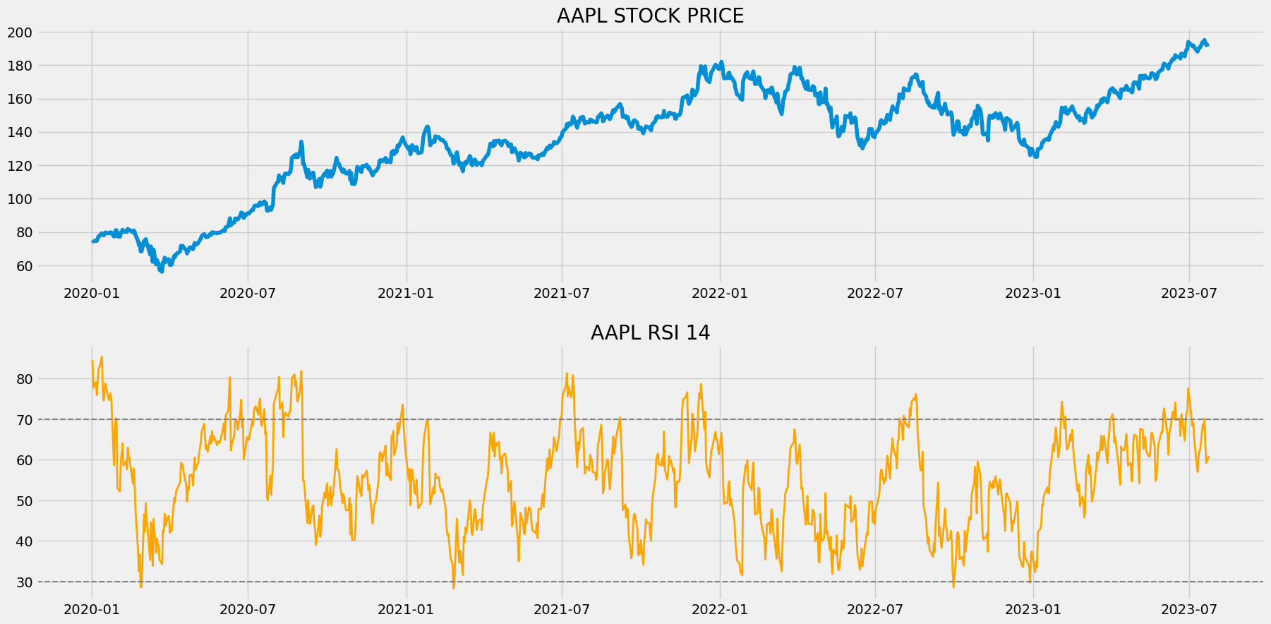
The above chart is separated into two panels: The above panel with the closing price of Apple and the lower panel with the calculated RSI 14 values of Apple. While analyzing the panel plotted with the RSI values, it can be seen that the trend and movement of the calculated values follow the same as the closing price of Apple. So, we can consider that RSI is a directional indicator. Some indicators are non-directional meaning that their movement will be inversely proportional to the actual stock movement and this can sometimes confuse traders and be hard to understand too.

While observing the RSI chart, we are able to see that the plot of RSI reveals trend reversals even before the market does. Simply speaking, the RSI shows a downtrend or an uptrend right before the actual market does. This shows that RSI is a leading indicator. A leading indicator is an indicator that takes into account the current value of a data series to predict future movements. RSI being a leading indicator helps in warning the traders about potential trend reversions before in time. The opposite of leading indicators is called lagging indicators. Lagging indicators are indicators that represent the current value by taking into account the historical values of a data series.

Trading Strategy

Now that we have built some basic understanding of the three indicators, let’s discuss the trading strategy that we are going to implement in this article. Basically, our strategy is a squeeze trading strategy which is confirmed by RSI. We will go long (buy the stock) whenever the Lower Keltner Channel is below the Lower Band, the Upper Keltner Channel is above the Upper Band, and the RSI shows a reading of below 30. Similarly, we go short (sell the stock) whenever the Lower Keltner Channel is below the Lower Band, the Upper Keltner Channel is above the Upper Band, and the RSI shows a reading of above 70. Our strategy can be represented as follows:

IF LOWER_KC < LOWER_BB AND UPPER_KC > UPPER_BB AND RSI < 30 ==> BUY
IF LOWER_KC < LOWER_BB AND UPPER_KC > UPPER_BB AND RSI > 70 ==> SELL

That’s it! This concludes our theory part and let’s move on to the programming part where we will use Python to first build the indicators from scratch, construct the discussed trading strategy, backtest the strategy on Apple stock data, and finally compare the results with that of SPY ETF. Let’s do some coding! Before moving on, a disclaimer: This article’s sole purpose is to educate people and must be considered as an information piece, but not as investment advice.

Implementation in Python

The coding part is classified into various steps as follows:

1. Importing Packages
2. Extracting Stock Data using EODHD
3. Bollinger Bands Calculation
4. Keltner Channel Calculation
5. RSI Calculation
6. Creating the Trading Strategy
7. Creating our Position
8. Backtesting
9. SPY ETF Comparison

We will be following the order mentioned in the above list and buckle up your seat belts to follow every upcoming coding part.

Step-1: Importing Packages

Importing the required packages into the Python environment is a non-skippable step. The primary packages are going to be Pandas to work with data, NumPy to work with arrays and for complex functions, Matplotlib for plotting purposes, and Requests to make API calls. The secondary packages are going to be Math for mathematical functions and Termcolor for font customization (optional).

Python Implementation:

# IMPORTING PACKAGES

import numpy as np
import requests
import pandas as pd
import matplotlib.pyplot as plt
from math import floor
from termcolor import colored as cl

plt.style.use('fivethirtyeight')
plt.rcParams['figure.figsize'] = (20,10)

Now that we have imported all the required packages into our Python. Let’s pull the historical data of Apple with EODHD’s OHLC split-adjusted data API endpoint.

Step-2: Extracting Stock Data using EODHD

In this step, we are going to pull the historical stock data of Apple using the OHLC split-adjusted API endpoint provided by EODHD. Before that, a note on EOD Historical Data: EOD Historical Data (EODHD) is a reliable provider of financial APIs covering a huge variety of market data ranging from historical data to economic and financial news data. Also, ensure that you have an EODHD account, only then you will be able to access your personal API key (a vital element to extract data with an API).

Python Implementation:

# EXTRACTING STOCK DATA

# EXTRACTING STOCK DATA

def get_historical_data(symbol, start_date):
    api_key = 'YOUR API KEY'
    api_url = f'https://eodhistoricaldata.com/api/technical/{symbol}?order=a&fmt=json&from={start_date}&function=splitadjusted&api_token={api_key}'
    raw_df = requests.get(api_url).json()
    df = pd.DataFrame(raw_df)
    df.date = pd.to_datetime(df.date)
    df = df.set_index('date')
    return df

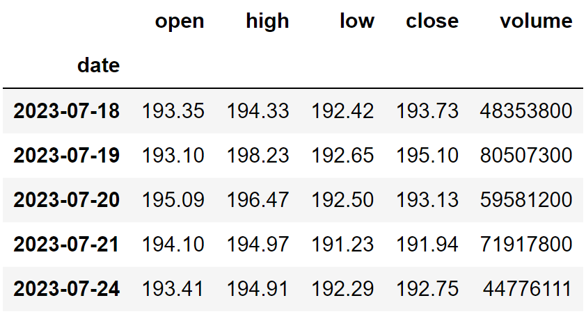
aapl = get_historical_data('AAPL', '2010-01-01')
aapl.tail()

Output:

Code Explanation: The first thing we did is to define a function named ‘get_historical_data’ that takes the stock’s symbol (‘symbol’) and the starting date of the historical data (‘start_date’) as parameters. Inside the function, we are defining the API key and the URL and stored them in their respective variable. Next, we are extracting the historical data in JSON format using the ‘get’ function and stored it in the ‘raw_df’ variable. After doing some processes to clean and format the raw JSON data, we are returning it in the form of a clean Pandas dataframe. Finally, we are calling the created function to pull the historic data of Apple from the start of 2010 and stored it into the ‘aapl’ variable.

Step-3: Bollinger Bands calculation

In this step, we are going to calculate the components of the Bollinger Bands by following the methods and formulas we discussed before.

Python Implementation:

# BOLLINGER BANDS CALCULATION

def sma(data, lookback):
    sma = data.rolling(lookback).mean()
    return sma

def get_bb(data, lookback):
    std = data.rolling(lookback).std()
    upper_bb = sma(data, lookback) + std * 2
    lower_bb = sma(data, lookback) - std * 2
    middle_bb = sma(data, lookback)
    return upper_bb, middle_bb, lower_bb

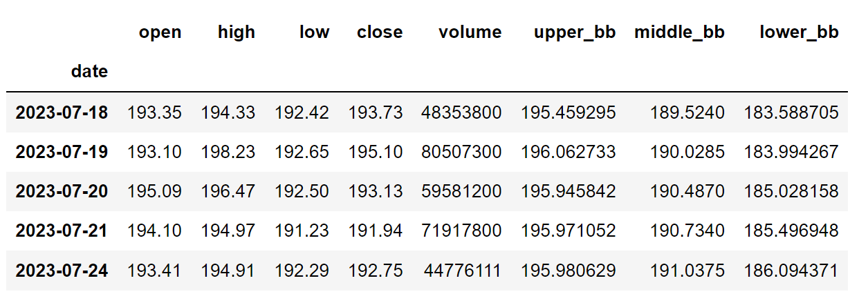
aapl['upper_bb'], aapl['middle_bb'], aapl['lower_bb'] = get_bb(aapl['close'], 20)
aapl.tail()

Output:

Code Explanation: The above can be classified into two parts: SMA calculation, and the Bollinger Bands calculation.

SMA calculation: Firstly, we are defining a function named ‘sma’ that takes the stock prices (‘data’), and the number of periods (‘lookback’) as the parameters. Inside the function, we are using the ‘rolling’ function provided by the Pandas package to calculate the SMA for the given number of periods. Finally, we are storing the calculated values in the ‘sma’ variable and returned them.

Bollinger Bands calculation: We are first defining a function named ‘get_bb’ that takes the stock prices (‘data’), and the number of periods as parameters (‘lookback’). Inside the function, we are using the ‘rolling’ and the ‘std’ function to calculate the standard deviation of the given stock data and stored the calculated standard deviation values in the ‘std’ variable. Next, we are calculating Bollinger Bands values using their respective formulas, and finally, we are returning the calculated values. We are storing the Bollinger Bands values into our ‘aapl’ dataframe using the created ‘bb’ function.

Step-4: Keltner Channel Calculation

In this step, we are going to calculate the components of the Keltner Channel indicator by following the methods we discussed before.

Python Implementation:

# KELTNER CHANNEL CALCULATION

def get_kc(high, low, close, kc_lookback, multiplier, atr_lookback):
    tr1 = pd.DataFrame(high - low)
    tr2 = pd.DataFrame(abs(high - close.shift()))
    tr3 = pd.DataFrame(abs(low - close.shift()))
    frames = [tr1, tr2, tr3]
    tr = pd.concat(frames, axis = 1, join = 'inner').max(axis = 1)
    atr = tr.ewm(alpha = 1/atr_lookback).mean()
    
    kc_middle = close.ewm(kc_lookback).mean()
    kc_upper = close.ewm(kc_lookback).mean() + multiplier * atr
    kc_lower = close.ewm(kc_lookback).mean() - multiplier * atr
    
    return kc_middle, kc_upper, kc_lower
    
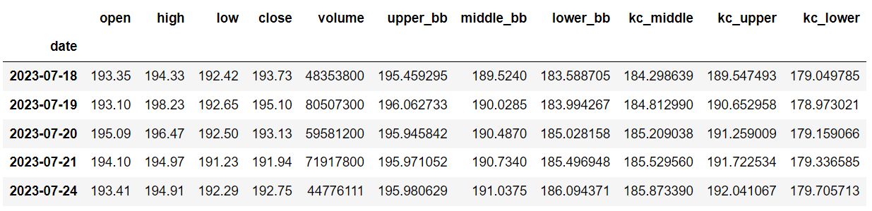
aapl['kc_middle'], aapl['kc_upper'], aapl['kc_lower'] = get_kc(aapl['high'], aapl['low'], aapl['close'], 20, 2, 10)
aapl.tail()

Output:

Code Explanation: We are first defining a function named ‘get_kc’ that takes a stock’s high (‘high’), low (‘low’), and closing price data (‘close’), the lookback period for the Keltner Channel (‘kc_lookback’), the multiplier value (‘multiplier), and the lookback period for the ATR (‘atr_lookback’) as parameters. The code inside the function can be separated into two parts: ATR calculation, and the Keltner Channel calculation.

ATR calculation: To determine the readings of the Average True Range, we are first calculating the three differences and storing them in their respective variables. Then we are combining all three differences into one dataframe using the ‘concat’ function and took the maximum values out of the three collective differences to determine the True Range. Then, using the ‘ewm’ and ‘mean’ functions, we are taking the customized Moving Average of True Range for a specified number of periods to get the ATR values.

Keltner Channel calculation: Utilizing the previously calculated ATR values, we are first calculating the middle line of the Keltner Channel by taking the EMA of ATR for a specified number of periods. Then comes the calculation of both the upper and lower bands. We are substituting the ATR values into the upper and lower bands formula we discussed before to get the readings of each of them. Finally, we are returning and calling the created function to get the Keltner Channel values of Apple.

Step-5: RSI Calculation

In this step, we are going to calculate the values of RSI with 14 as the lookback period using the RSI formula we discussed before.

Python Implementation:

# RSI CALCULATION
def get_rsi(close, lookback):
    ret = close.diff()
    up = []
    down = []
    for i in range(len(ret)):
        if ret[i] < 0:
            up.append(0)
            down.append(ret[i])
        else:
            up.append(ret[i])
            down.append(0)
    up_series = pd.Series(up)
    down_series = pd.Series(down).abs()
    up_ewm = up_series.ewm(com = lookback - 1, adjust = False).mean()
    down_ewm = down_series.ewm(com = lookback - 1, adjust = False).mean()
    rs = up_ewm/down_ewm
    rsi = 100 - (100 / (1 + rs))
    rsi_df = pd.DataFrame(rsi).rename(columns = {0:'rsi'}).set_index(close.index)
    rsi_df = rsi_df.dropna()
    return rsi_df[3:]

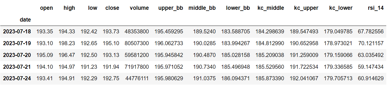
aapl['rsi_14'] = get_rsi(aapl['close'], 14)
aapl = aapl.dropna()
aapl.tail()

Output:

Code Explanation: Firstly, we are defining a function named ‘get_rsi’ that takes the closing price of a stock (‘close’) and the lookback period (‘lookback’) as parameters. Inside the function, we are first calculating the returns of the stock using the ‘diff’ function provided by the Pandas package and stored it in the ‘ret’ variable. This function basically subtracts the current value from the previous value. Next, we are passing a for-loop on the ‘ret’ variable to distinguish gains from losses and append those values to the concerning variable (‘up’ or ‘down’).

Then, we are calculating the Exponential Moving Averages for both the ‘up’ and ‘down’ using the ‘ewm’ function provided by the Pandas package and storing them in the ‘up_ewm’ and ‘down_ewm’ variables respectively. Using these calculated EMAs, we are determining the Relative Strength by following the formula we discussed before and storing it into the ‘rs’ variable.

By making use of the calculated Relative Strength values, we are calculating the RSI values by following its formula. After doing some data processing and manipulations, we are returning the calculated Relative Strength Index values in the form of a Pandas dataframe. Finally, we are calling the created function to store the RSI values of Apple with 14 as the lookback period.

Step-6: Creating the Trading Strategy:

In this step, we are going to implement the discussed Bollinger Bands, Keltner Channel, and Relative Strength Index trading strategy in Python.

Python Implementation:

# TRADING STRATEGY

def bb_kc_rsi_strategy(prices, upper_bb, lower_bb, kc_upper, kc_lower, rsi):
    buy_price = []
    sell_price = []
    bb_kc_rsi_signal = []
    signal = 0
    
    for i in range(len(prices)):
        if lower_bb[i] < kc_lower[i] and upper_bb[i] > kc_upper[i] and rsi[i] < 30:
            if signal != 1:
                buy_price.append(prices[i])
                sell_price.append(np.nan)
                signal = 1
                bb_kc_rsi_signal.append(signal)
            else:
                buy_price.append(np.nan)
                sell_price.append(np.nan)
                bb_kc_rsi_signal.append(0)
                
        elif lower_bb[i] < kc_lower[i] and upper_bb[i] > kc_upper[i] and rsi[i] > 70:
            if signal != -1:
                buy_price.append(np.nan)
                sell_price.append(prices[i])
                signal = -1
                bb_kc_rsi_signal.append(signal)
            else:
                buy_price.append(np.nan)
                sell_price.append(np.nan)
                bb_kc_rsi_signal.append(0)
        else:
            buy_price.append(np.nan)
            sell_price.append(np.nan)
            bb_kc_rsi_signal.append(0)
                        
    return buy_price, sell_price, bb_kc_rsi_signal

buy_price, sell_price, bb_kc_rsi_signal = bb_kc_rsi_strategy(aapl['close'], aapl['upper_bb'], aapl['lower_bb'], aapl['kc_upper'], aapl['kc_lower'], aapl['rsi_14'])

Code Explanation: First, we are defining a function named ‘bb_kc_rsi_strategy’ which takes the stock prices (‘prices’), Upper Keltner Channel (‘kc_upper’), Lower Keltner Channel (‘kc_lower’), Upper Bollinger band (‘upper_bb’), Lower Bollinger band (‘lower_bb’), and the Relative Strength Index readings (‘rsi’) as parameters.

Inside the function, we are creating three empty lists (buy_price, sell_price, and bb_kc_rsi_signal) in which the values will be appended while creating the trading strategy.

After that, we are implementing the trading strategy through a for-loop. Inside the for-loop, we are passing certain conditions, and if the conditions are satisfied, the respective values will be appended to the empty lists. If the condition to buy the stock gets satisfied, the buying price will be appended to the ‘buy_price’ list, and the signal value will be appended as 1 representing buying the stock. Similarly, if the condition to sell the stock gets satisfied, the selling price will be appended to the ‘sell_price’ list, and the signal value will be appended as -1 representing to sell the stock. Finally, we are returning the lists appended with values. Then, we are calling the created function and stored the values in their respective variables.

Step-7: Creating our Position

In this step, we are going to create a list that indicates 1 if we hold the stock or 0 if we don’t own or hold the stock.

Python Implementation:

# POSITION

position = []
for i in range(len(bb_kc_rsi_signal)):
    if bb_kc_rsi_signal[i] > 1:
        position.append(0)
    else:
        position.append(1)
        
for i in range(len(aapl['close'])):
    if bb_kc_rsi_signal[i] == 1:
        position[i] = 1
    elif bb_kc_rsi_signal[i] == -1:
        position[i] = 0
    else:
        position[i] = position[i-1]
        
kc_upper = aapl['kc_upper']
kc_lower = aapl['kc_lower']
upper_bb = aapl['upper_bb'] 
lower_bb = aapl['lower_bb']
rsi = aapl['rsi_14']
close_price = aapl['close']
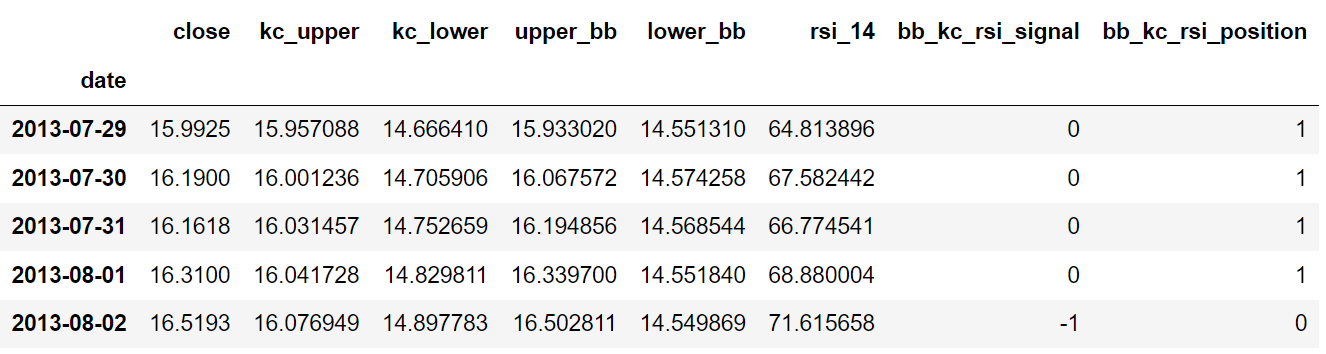
bb_kc_rsi_signal = pd.DataFrame(bb_kc_rsi_signal).rename(columns = {0:'bb_kc_rsi_signal'}).set_index(aapl.index)
position = pd.DataFrame(position).rename(columns = {0:'bb_kc_rsi_position'}).set_index(aapl.index)

frames = [close_price, kc_upper, kc_lower, upper_bb, lower_bb, rsi, bb_kc_rsi_signal, position]
strategy = pd.concat(frames, join = 'inner', axis = 1)

Output:

Code Explanation: First, we are creating an empty list named ‘position’. We are passing two for-loops, one is to generate values for the ‘position’ list to just match the length of the ‘signal’ list. The other for-loop is the one we are using to generate actual position values.

Inside the second for-loop, we are iterating over the values of the ‘signal’ list, and the values of the ‘position’ list get appended concerning which condition gets satisfied. The value of the position remains 1 if we hold the stock or remains 0 if we sold or don’t own the stock. Finally, we are doing some data manipulations to combine all the created lists into one dataframe.

From the output being shown, we can see that in the first four rows, our position in the stock has remained at 1 (since there isn’t any change in the trading signal) but our position suddenly turned to 0 as we sold the stock when the trading signal represents a buy signal (-1). Our position will remain -1 until some changes in the trading signal occur. Now it’s time to implement some backtesting processes!

Step-8: Backtesting

Before moving on, it is essential to know what backtesting is. Backtesting is the process of seeing how well our trading strategy has performed on given stock data. In our case, we are going to implement a backtesting process for our trading strategy over the Apple stock data.

Python Implementation:

# BACKTESTING

aapl_ret = pd.DataFrame(np.diff(aapl['close'])).rename(columns = {0:'returns'})
bb_kc_rsi_strategy_ret = []

for i in range(len(aapl_ret)):
    returns = aapl_ret['returns'][i]*strategy['bb_kc_rsi_position'][i]
    bb_kc_rsi_strategy_ret.append(returns)
    
bb_kc_rsi_strategy_ret_df = pd.DataFrame(bb_kc_rsi_strategy_ret).rename(columns = {0:'bb_kc_rsi_returns'})
investment_value = 100000
bb_kc_rsi_investment_ret = []

for i in range(len(bb_kc_rsi_strategy_ret_df['bb_kc_rsi_returns'])):
    number_of_stocks = floor(investment_value/aapl['close'][i])
    returns = number_of_stocks*bb_kc_rsi_strategy_ret_df['bb_kc_rsi_returns'][i]
    bb_kc_rsi_investment_ret.append(returns)

bb_kc_rsi_investment_ret_df = pd.DataFrame(bb_kc_rsi_investment_ret).rename(columns = {0:'investment_returns'})
total_investment_ret = round(sum(bb_kc_rsi_investment_ret_df['investment_returns']), 2)
profit_percentage = floor((total_investment_ret/investment_value)*100)
print(cl('Profit gained from the BB KC RSI strategy by investing $100k in AAPL : {}'.format(total_investment_ret), attrs = ['bold']))
print(cl('Profit percentage of the BB KC RSI strategy : {}%'.format(profit_percentage), attrs = ['bold']))

Output:

Profit gained from the BB KC RSI strategy by investing $100k in AAPL : 165737.51
Profit percentage of the BB KC RSI strategy : 165%

Code Explanation: First, we are calculating the returns of the Apple stock using the ‘diff’ function provided by the NumPy package and we have stored it as a dataframe in the ‘aapl_ret’ variable. Next, we are passing a for-loop to iterate over the values of the ‘aapl_ret’ variable to calculate the returns we gained from our RVI trading strategy, and these returns values are appended to the ‘bb_kc_rsi_strategy_ret’ list. Next, we are converting the ‘bb_kc_rsi_strategy_ret’ list into a dataframe and storing it into the ‘bb_kc_rsi_strategy_ret_df’ variable.

Next comes the backtesting process. We are going to backtest our strategy by investing a hundred thousand USD into our trading strategy. So first, we are storing the amount of investment into the ‘investment_value’ variable. After that, we are calculating the number of Apple stocks we can buy using the investment amount. You can notice that I’ve used the ‘floor’ function provided by the Math package because, while dividing the investment amount by the closing price of Apple stock, it spits out an output with decimal numbers. The number of stocks should be an integer but not a decimal number. Using the ‘floor’ function, we can cut out the decimals. Remember that the ‘floor’ function is way more complex than the ‘round’ function. Then, we are passing a for-loop to find the investment returns followed by some data manipulation tasks.

Finally, we are printing the total return we got by investing a hundred thousand into our trading strategy and it is revealed that we have made an approximate profit of 165K USD in around thirteen-and-a-half years with a profit percentage of 165%. That’s great! Now, let’s compare our returns with SPY ETF (an ETF designed to track the S&P 500 stock market index) returns.

Step-8: SPY ETF Comparison

This step is optional but it is highly recommended as we can get an idea of how well our trading strategy performs against a benchmark (SPY ETF). In this step, we will extract the SPY ETF data using the ‘get_historical_data’ function we created and compare the returns we get from the SPY ETF with our trading strategy returns on Apple.

Python Implementation:

# SPY ETF COMPARISON

def get_benchmark(start_date, investment_value):
    spy = get_historical_data('SPY', start_date)['close']
    benchmark = pd.DataFrame(np.diff(spy)).rename(columns = {0:'benchmark_returns'})
    
    investment_value = investment_value
    benchmark_investment_ret = []
    
    for i in range(len(benchmark['benchmark_returns'])):
        number_of_stocks = floor(investment_value/spy[i])
        returns = number_of_stocks*benchmark['benchmark_returns'][i]
        benchmark_investment_ret.append(returns)

    benchmark_investment_ret_df = pd.DataFrame(benchmark_investment_ret).rename(columns = {0:'investment_returns'})
    return benchmark_investment_ret_df

benchmark = get_benchmark('2010-01-01', 100000)
investment_value = 100000
total_benchmark_investment_ret = round(sum(benchmark['investment_returns']), 2)
benchmark_profit_percentage = floor((total_benchmark_investment_ret/investment_value)*100)
print(cl('Benchmark profit by investing $100k : {}'.format(total_benchmark_investment_ret), attrs = ['bold']))
print(cl('Benchmark Profit percentage : {}%'.format(benchmark_profit_percentage), attrs = ['bold']))
print(cl('BB KC RSI Strategy profit is {}% higher than the Benchmark Profit'.format(profit_percentage - benchmark_profit_percentage), attrs = ['bold']))

Output:

Benchmark profit by investing $100k : 159541.51
Benchmark Profit percentage : 159%
BB KC RSI Strategy profit is 6% higher than the Benchmark Profit

Code Explanation: The code used in this step is almost similar to the one used in the previous backtesting step but, instead of investing in Apple, we are investing in SPY ETF by not implementing any trading strategies. From the output, we can see that our trading strategy has outperformed the SPY ETF by 6%. That’s awesome!

Final Thoughts!

After the immense process of crushing both theory and coding parts, we have successfully learned what the three indicators are all about and built a killer trading strategy out of them that manages to surpass the returns of the SPY ETF in a 13-year timeframe. From the results, it is notable that by consolidating two or more indicators, we can gain better returns out of our investment than we could with a single indicator trading strategy. Also, we can erase non-authentic signals from our strategy as much as possible.

With that being said, you’ve reached the end of the article. Hope you learned something new and useful from this article!

Bollinger Bands

Keltner Channel (KC)

Relative Strength Index

Trading Strategy

Implementation in Python

Step-1: Importing Packages

Step-2: Extracting Stock Data using EODHD

Step-3: Bollinger Bands calculation

Step-4: Keltner Channel Calculation

Step-5: RSI Calculation

Step-6: Creating the Trading Strategy:

Step-7: Creating our Position

Step-8: Backtesting

Step-8: SPY ETF Comparison

Final Thoughts!

Related Articles

Backtesting Technical Analysis Strategies with Excel(SMA, RSI, MACD)

Practical Guide to Automated Detection Trading Patterns with Python

Backtesting a Killer Mean Reversion Trading Strategy with Python

Maximising Profits Trading with Moving Average Crossovers

How to Use DMI and ADX of the Technical Indicators API with Python

Implementing a Candlestick Momentum Strategy in Python