

Trading can be a highly emotional experience. It can significantly disrupt your progress if you can’t manage your emotions. That’s why experienced trading professionals (not just those who claim to be experts online) consistently stress one key principle: thoroughly backtest your strategies and strive to separate your emotions from your decision-making process.
But let’s be honest: it’s hard to stay completely unemotional, especially when reacting to news events. This raises an interesting question: can we actually measure the market’s emotional response to news and use that data to inform our trading decisions?
Before we get started, it’s important to clarify that this article isn’t about handing you a ready-made trading strategy to use tomorrow. Instead, my aim is to demonstrate that sentiment can, in fact, be quantified and applied across different types of automation. And here’s a hint : the answer is a resounding YES!
How can the EODHD API for sentiment help us?
Well, EODHD can’t help us control our emotions, but it can definitely help us gauge the emotions of others.
EODHD provides an API that delivers daily sentiment scores for major stocks, ETFs, and cryptocurrencies by analysing both news sources and social media. These sentiment scores are normalised on a scale from -1, representing very negative sentiment, to 1, indicating very positive sentiment. This allows traders and analysts to quantify and incorporate market sentiment into their trading strategies.
Let’s check out some data.
First, we start with the imports and parameters. We will initially use Apple stock prices for the last two years.
import requests
import pandas as pd
import numpy as np
import matplotlib.pyplot as plt
import os
from datetime import datetime, timedelta
import seaborn as sns

api_token = os.environ.get('EODHD_API_TOKEN')

TICKER = 'AAPL.US'
# Using a 2-year period for analysis
end_date = datetime.now()
start_date = end_date - timedelta(days=730)
from_date = start_date.strftime('%Y-%m-%d')
to_date = end_date.strftime('%Y-%m-%d')
In the second step, we will retrieve the price from the EODHD API.
def get_price_data(ticker, from_date, to_date):
    url = f'https://eodhd.com/api/eod/{ticker}'
    query = {'api_token': api_token, 'fmt': 'json', 'from': from_date, 'to': to_date}
    response = requests.get(url, params=query)
    if response.status_code != 200:
            print(f"Error retrieving price data: {response.status_code}")
            print(response.text)
            return None
    price_data = response.json()
    price_df = pd.DataFrame(price_data)
    # Convert date string to datetime for easier manipulation
    price_df['date'] = pd.to_datetime(price_df['date'])
    # Set date as index
    price_df.set_index('date', inplace=True)
    # Sort by date (ascending)
    price_df.sort_index(inplace=True)
    return price_df
price_df = get_price_data(TICKER, from_date, to_date)
price_df['pct_change'] = price_df['adjusted_close'].pct_change() * 100
And then, using the EODHD API for sentiment, we’ll gather the sentiment data.
def get_sentiment_data(ticker, from_date, to_date):
    url = f'https://eodhd.com/api/sentiments'
    query = {'api_token': api_token, 's': ticker, 'from': from_date, 'to': to_date, 'fmt': 'json'}
    response = requests.get(url, params=query)
    if response.status_code != 200:
            print(f"Error retrieving sentiment data: {response.status_code}")
            print(response.text)
            return None
    sentiment_data = response.json()
    # Access the sentiment data using the ticker symbol as a key
    sentiment_df = pd.DataFrame(sentiment_data[ticker])
    # Convert date string to datetime
    sentiment_df['date'] = pd.to_datetime(sentiment_df['date'])
    # Set date as index
    sentiment_df.set_index('date', inplace=True)
    # Sort by date (ascending)
    sentiment_df.sort_index(inplace=True)
    # Rename column normalized to sentiment
    sentiment_df.rename(columns={'normalized': 'sentiment'}, inplace=True)
    return sentiment_df
sentiment_df = get_sentiment_data(TICKER, from_date, to_date)
For this analysis, the daily sentiment column is our main indicator. I’ll start by combining all the sentiment data into a single dataframe, making it easier to analyse trends across different assets. To highlight the underlying trend, I’ll calculate a rolling average and remove any outliers from the data. This approach ensures the resulting trend line is both clear and visually distinct, allowing us to better observe sentiment shifts over time.
merged_df = pd.merge(
    price_df[['adjusted_close','pct_change']],
    sentiment_df[['sentiment']],
    left_index=True,
    right_index=True,
    how='inner'
)

# Rename columns for clarity
merged_df.columns = ['price', 'price_pct_change', 'sentiment']
clean_df = merged_df[['price_pct_change','sentiment']].dropna().replace([np.inf, -np.inf], np.nan).dropna()
# Calculate IQR and bounds for both variables
def remove_outliers(df, columns):
    df_clean = df.copy()
    for column in columns:
        Q1 = df[column].quantile(0.25)
        Q3 = df[column].quantile(0.75)
        IQR = Q3 - Q1
        lower_bound = Q1 - 1.5 * IQR
        upper_bound = Q3 + 1.5 * IQR
        df_clean = df_clean[df_clean[column].between(lower_bound, upper_bound)]
    return df_clean
# Apply outlier removal
clean_df = remove_outliers(clean_df, ['price_pct_change', 'sentiment'])

# Create a scatter plot to visualize the relationship
plt.figure(figsize=(10, 6))
plt.scatter(clean_df['sentiment'], clean_df['price_pct_change'], alpha=0.6)
plt.xlabel('Sentiment Change')
plt.ylabel('Daily Price Percentage Change (%)')
plt.grid(True)
# Add a trend line
if len(clean_df) > 1:  # Only add trend line if we have enough data points
    try:
        z = np.polyfit(clean_df['sentiment'], clean_df['price_pct_change'], 1)
        p = np.poly1d(z)
        plt.plot(sorted(clean_df['sentiment']), p(sorted(clean_df['sentiment'])), "r--", alpha=0.8)
    except np.linalg.LinAlgError as e:
        print(f"Could not fit trend line: {e}")
plt.tight_layout()
plt.show()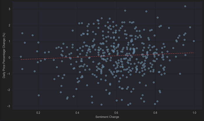
Interestingly, even though the trend line isn’t particularly steep, it clearly points upward, reflecting the impact of increasingly positive news sentiment on daily price movements. In short, positive news tends to correlate with more substantial returns.
Of course, this insight only becomes actionable when we translate it into a practical strategy. So, let’s dive into building one!
Moving Average Sentiment Strategy
I’ll use a straightforward slow-fast moving-average strategy applied to both price and sentiment data. This generates two distinct strategy variations:
Strategy 1: LONGSHORT
- Long Entry: When both price and sentiment fast MAs cross above their slow MAs (confirming bullish alignment).
- Short Entry: When both slow MAs exceed their fast counterparts (confirming bearish alignment).
- Neutral: When price and sentiment signals disagree.
Strategy 2: ALWAYSLONG_OUTWHEN_NEGSENT
- Long Entry: Always hold long positions when the sentiment’s fast MA is above its slow MA.
- Exit: Immediately close positions when sentiment’s fast MA drops below its slow MA.
Implementation Workflow
We’ll define two core functions:
- Equity Curve Calculation: Quantifies strategy performance over time.
- Signal Execution: Translates MA crossovers into trade actions.
This code transforms quantified sentiment into actionable signals while systematically minimising emotional interference.
First the equity curve:
def calculate_equity_curve(prices, signals):
    # Ensure index alignment
    signals = signals.shift(1)  # Shift signals to align with the period for trade execution
    signals = signals.reindex(prices.index).fillna(0)
    # Calculate percentage changes
    pct_changes = prices.pct_change().fillna(0)
    # Calculate equity curve
    equity_curve = (1 + pct_changes * signals).cumprod() * 100
    return equity_curve
And then the actual strategy:
def analyze_ma_crossover_strategy(ticker, fast_window, slow_window, from_date, to_date, strategy_type = "LONGSHORT"):

    # Retrieve price data
    price_df = get_price_data(ticker, from_date, to_date)
    if price_df is None or len(price_df) == 0:
        print(f"Error: Could not retrieve price data for {ticker}")
        return None
    # Retrieve sentiment data
    sentiment_df = get_sentiment_data(ticker, from_date, to_date)
    if sentiment_df is None or len(sentiment_df) == 0:
        print(f"Error: Could not retrieve sentiment data for {ticker}")
        return None
    # Create a combined dataframe
    df = pd.DataFrame(index=price_df.index)
    df['adjusted_close'] = price_df['adjusted_close']
    # Merge sentiment data (may have different dates)
    df = df.join(sentiment_df['sentiment'], how='left')
    # Forward fill missing sentiment values
    df['sentiment'] = df['sentiment'].ffill()
    # Calculate moving averages for price
    df[f'price_fast_ma'] = df['adjusted_close'].rolling(window=fast_window).mean()
    df[f'price_slow_ma'] = df['adjusted_close'].rolling(window=slow_window).mean()
    # Calculate moving averages for sentiment
    df[f'sentiment_fast_ma'] = df['sentiment'].rolling(window=fast_window).mean()
    df[f'sentiment_slow_ma'] = df['sentiment'].rolling(window=slow_window).mean()
    # Generate signals
    if strategy_type == "LONGSHORT":
        # 1 when fast MA > slow MA for both price and sentiment
        # -1 when fast MA < slow MA for both price and sentiment
        # 0 otherwise
        df['price_signal'] = np.where(df[f'price_fast_ma'] > df[f'price_slow_ma'], 1, -1)
        df['sentiment_signal'] = np.where(df[f'sentiment_fast_ma'] > df[f'sentiment_slow_ma'], 1, -1)
        df['signal'] = np.where((df['price_signal'] == 1) & (df['sentiment_signal'] == 1), 1,
                               np.where((df['price_signal'] == -1) & (df['sentiment_signal'] == -1), -1, 0))
    elif strategy_type == 'ALWAYSLONG_OUTWHEN_NEGSENT':
        # Always 1 except when sentiment signal is
        df['price_signal'] = pd.Series(1, index=df.index)
        df['sentiment_signal'] = np.where(df[f'sentiment_fast_ma'] > df[f'sentiment_slow_ma'], 1, -1)
        df['signal'] = np.where((df['sentiment_signal'] == -1), 0, df[f'price_signal'])
    else:
        raise ValueError("Invalid strategy type")
    # Calculate returns
    df['pct_change'] = df['adjusted_close'].pct_change().fillna(0)
    # Calculate equity curves using the calculate_equity_curve function
    # For buy and hold, we use a signal of 1 (always long)
    buy_hold_signal = pd.Series(1, index=df.index)
    df['buy_hold_equity'] = calculate_equity_curve(df['adjusted_close'], buy_hold_signal) / 100
    # For strategy equity, we use the generated signals
    df['strategy_equity'] = calculate_equity_curve(df['adjusted_close'], df['signal']) / 100
    return df
We’ll implement the LONSHORT strategy with a 5-day fast and 15-day slow window for price and sentiment moving averages. After generating the signals, we’ll visualise the results in a performance plot to assess effectiveness.
Here’s a hands-on test that shows how combining quantified sentiment with technical indicators produces actionable trading signals. Let’s see how it performs!
def plot_strategy_results(df):
    # Create a figure with single plot for equity curves
    plt.figure(figsize=(12, 6))
    # Plot equity curves
    plt.plot(df.index, df['buy_hold_equity'], label='Buy & Hold')
    plt.plot(df.index, df['strategy_equity'], label='MA Crossover Strategy')
    plt.title('Equity Curves')
    plt.ylabel('Equity (Starting at 1)')
    plt.xlabel('Date')
    plt.legend()
    plt.grid(True)
    plt.tight_layout()
    plt.show()
result_df = analyze_ma_crossover_strategy(TICKER, fast_window=5, slow_window=15, from_date=from_date, to_date=to_date, strategy_type="LONGSHORT")
plot_strategy_results(result_df)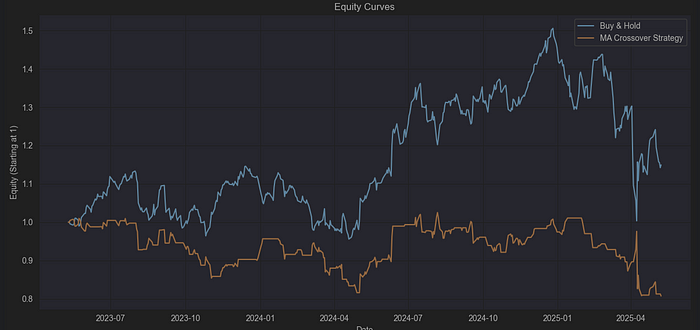
The outcome is underwhelming . This approach failed to capture the mid-2024 uptrend and ultimately led to losses. To address this, let’s tighten the moving average windows to 1 and 5 and apply the second strategy variation for a fresh perspective.
result_df = analyze_ma_crossover_strategy(TICKER, fast_window=1, slow_window=5, from_date=from_date, to_date=to_date, strategy_type="ALWAYSLONG_OUTWHEN_NEGSENT")
plot_strategy_results(result_df)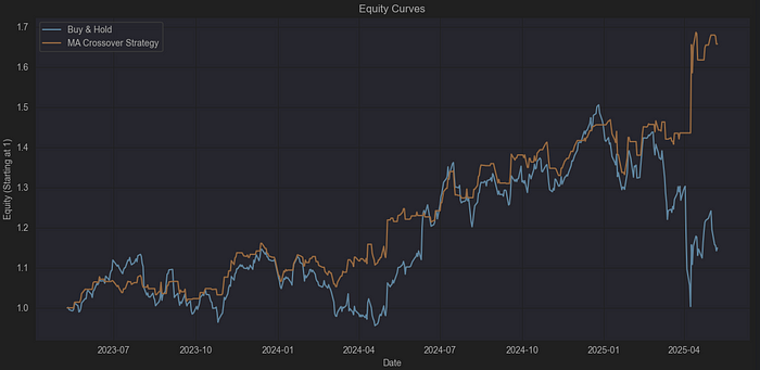
This time, the strategy’s performance improved noticeably. The key advantage came from remaining neutral in the days immediately following the US tariff announcements — a period when buy-and-hold investors suffered significant losses. By avoiding exposure during this volatile window and then leveraging the surge in positive sentiment that followed, the strategy was able to deliver strong returns.
Who said overfitting is bad?
Absolutely, I’m aware that overfitting is undesirable. However, it can sometimes help uncover patterns, reinforcing our core idea: news sentiment is quantifiable! We are going to work with stocks from various sectors. Practically, we will use the functions developed before to calculate the returns.
tickers = ['AAPL.US', 'MSFT.US', 'NVDA.US', 'GOOGL.US', 'META.US', 'AMZN.US', 'TSLA.US', 'HD.US', 'JNJ.US', 'UNH.US', 'PFE.US', 'MRK.US', 'JPM.US', 'V.US', 'MA.US', 'PG.US', 'KO.US', 'PEP.US', 'XOM.US', 'CVX.US', 'NEE.US', 'DUK.US', 'LIN.US', 'BA.US', 'CAT.US', 'RTX.US', 'SPG.US', 'AMT.US', 'MO.US']
# Create lists to store the data
data = []
fast_windows = range(1, 6)  # 1 to 5
slow_windows = range(5, 21, 5)  # 5, 10, 15, 20

# Loop through each ticker
for ticker in tickers:
    # Initialize variables to track the best parameters and results for this ticker
    best_fast_window = None
    best_slow_window = None
    best_strategy_type = None
    best_return = -float('inf')
    best_buy_hold_return = None
    # Rest of the loop logic remains the same...
    for fast_window in fast_windows:
        for slow_window in slow_windows:
            for strategy_type in ["LONGSHORT", "ALWAYSLONG_OUTWHEN_NEGSENT"]:
                if fast_window >= slow_window:
                    continue
                result_df = analyze_ma_crossover_strategy(ticker, fast_window, slow_window,
                                                          from_date=from_date, to_date=to_date,
                                                          strategy_type=strategy_type)
                if result_df is not None:
                    strategy_return = result_df['strategy_equity'].iloc[-1]
                    buy_hold_return = result_df['buy_hold_equity'].iloc[-1]
                    if strategy_return > best_return:
                        best_return = strategy_return
                        best_fast_window = fast_window
                        best_slow_window = slow_window
                        best_strategy_type = strategy_type
                        best_buy_hold_return = buy_hold_return
    # Instead of concatenating each time, append to the list
    data.append({
        'ticker': ticker,
        'fast_window': best_fast_window,
        'slow_window': best_slow_window,
        'strategy_type': best_strategy_type,
        'strategy_return': best_return,
        'buy_hold_return': best_buy_hold_return
    })
# Create the DataFrame once with all the data
optimal_params_df = pd.DataFrame(data)
optimal_params_df['str_bnh_diff'] = optimal_params_df['strategy_return'] - optimal_params_df['buy_hold_return']
optimal_params_df
Now let’s plot the results.
plt.figure(figsize=(12, 10))
# Create horizontal bar positions
y_pos = np.arange(len(optimal_params_df))
# Create color array for strategy returns based on comparison with buy & hold
strategy_colors = ['green' if s > b else 'red' for s, b in zip(optimal_params_df['strategy_return'], optimal_params_df['buy_hold_return'])]
# Plot the bars with new colors
plt.barh(y_pos - 0.2, optimal_params_df['strategy_return'], height=0.4, label='Strategy Return', color=strategy_colors)
plt.barh(y_pos + 0.2, optimal_params_df['buy_hold_return'], height=0.4, label='Buy & Hold Return', color='grey')
plt.yticks(y_pos, optimal_params_df['ticker'])
plt.xlabel('Return')
plt.title('Strategy vs Buy & Hold Returns by Ticker')
plt.legend()
plt.grid(True, alpha=0.3)
plt.tight_layout()
plt.show()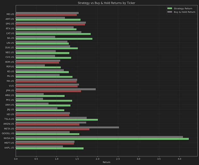
Most of our strategy variations beat the buy-and-hold approach, as shown by the green returns in our analysis. What’s notable is that every asset that lost money under buy-and-hold made at least some gains using our method, and some actually lost no money at all.
Before wrapping up, I’ll skip optimisation and instead compile every possible combination of fast and slow windows. This complete dataset will be visualised as a heatmap, directly comparing the effectiveness of window pairs across all tested parameters.
This transparent approach avoids cherry-picking and reveals the full spectrum of strategy performance.
tickers = ['AAPL.US', 'MSFT.US', 'NVDA.US', 'GOOGL.US', 'META.US', 'AMZN.US', 'TSLA.US', 'HD.US', 'JNJ.US', 'UNH.US', 'PFE.US', 'MRK.US', 'JPM.US', 'V.US', 'MA.US', 'PG.US', 'KO.US', 'PEP.US', 'XOM.US', 'CVX.US', 'NEE.US', 'DUK.US', 'LIN.US', 'BA.US', 'CAT.US', 'RTX.US', 'SPG.US', 'AMT.US', 'MO.US']
# Create lists to store the data
data = []
fast_windows = range(1, 6)  # 1 to 5
slow_windows = range(5, 21, 5)  # 5, 10, 15, 20

# Loop through each ticker
for ticker in tickers:
    # Initialize variables to track the best parameters and results for this ticker
    best_fast_window = None
    best_slow_window = None
    best_strategy_type = None
    best_return = -float('inf')
    best_buy_hold_return = None
    # Rest of the loop logic remains the same...
    for fast_window in fast_windows:
        for slow_window in slow_windows:
            for strategy_type in ["LONGSHORT", "ALWAYSLONG_OUTWHEN_NEGSENT"]:
                if fast_window >= slow_window:
                    continue
                result_df = analyze_ma_crossover_strategy(ticker, fast_window, slow_window,
                                                          from_date=from_date, to_date=to_date,
                                                          strategy_type=strategy_type)
                if result_df is not None:
                    strategy_return = result_df['strategy_equity'].iloc[-1]
                    buy_hold_return = result_df['buy_hold_equity'].iloc[-1]
                    data.append({
                        'ticker': ticker,
                        'fast_window': fast_window,
                        'slow_window': slow_window,
                        'strategy_type': strategy_type,
                        'strategy_return': strategy_return,
                        'buy_hold_return': buy_hold_return
                    })
# Create the DataFrame once with all the data
all_runs_df = pd.DataFrame(data)
all_runs_df['str_bnh_diff'] = optimal_params_df['strategy_return'] - optimal_params_df['buy_hold_return']
# First, let's create the aggregated data
grouped_df = all_runs_df.groupby(['fast_window', 'slow_window', 'strategy_type']).agg({
    'strategy_return': 'mean',
    'buy_hold_return': 'mean',
}).reset_index()
# Calculate the difference for coloring
grouped_df['str_bnh_diff'] = grouped_df['strategy_return'] - grouped_df['buy_hold_return']
plt.figure(figsize=(12, 8))
# Pivot the data to create a matrix suitable for heatmap
heatmap_data = grouped_df.pivot_table(
    index='fast_window',
    columns='slow_window',
    values='str_bnh_diff',
    aggfunc='mean'
)
# Create heatmap
sns.heatmap(heatmap_data,
            annot=True,
            fmt='.2f',
            cmap='RdYlGn',
            center=0,
            cbar_kws={'label': 'Strategy Return - Buy & Hold Return'}
            )
plt.title('Strategy Performance by Window Combinations')
plt.xlabel('Slow Window')
plt.ylabel('Fast Window')
plt.tight_layout()
plt.show()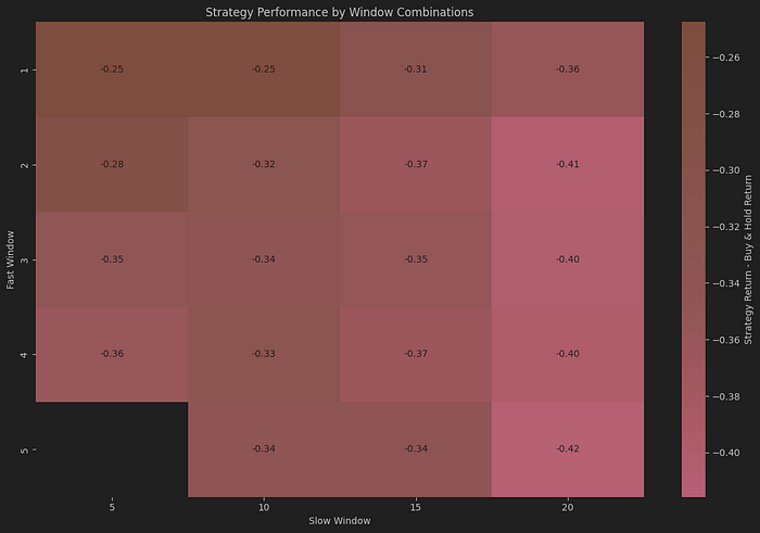
The heatmap reveals two key insights:
First, while optimising the fast and slow windows for each stock individually produced encouraging results, the strategy underperforms buy-and-hold on average across all stocks. This suggests that sensitivity to news sentiment varies significantly between different assets.
Second, it’s clear that setting the fast window to 1 — essentially using the previous day’s sentiment — consistently outperforms strategies with larger window sizes. This highlights the immediate impact of news sentiment on short-term price movements.
Conclusion and food for thought
To wrap up, here are a few key takeaways:
- Sentiment scores extracted from news and social media can be quantified and integrated into trading strategies, and they show a clear positive correlation with daily price movements.
- Tailoring moving average windows to individual stocks often led to better results than a buy-and-hold approach, especially for assets that typically underperform.
- Some stocks are inherently more responsive to news events than others.
- Speed matters . Comparing yesterday’s sentiment with the previous five-day average consistently delivered the most substantial returns, underscoring how quickly news impacts the market.
- The EODHD API effectively captured major market shocks, such as the US tariff announcements, helping the strategy avoid significant drawdowns1.
If you’re interested in exploring this area further, consider these ideas:
- Investigate how historical sentiment trends relate to multi-day returns, rather than focusing solely on daily changes.
- Analyse the volatility of sentiment and see if it correlates with trading volume.
- Identify sideways or ranging markets and examine whether sentiment remains flat during these periods.
- Look for patterns in asset sensitivity to news and explore the reasons behind these differences.