Benchmark Tracking and Cointegration Analysis with Python

Cointegration analysis is a sophisticated statistical approach widely used in the field of financial time series analysis. It’s particularly useful for identifying and analyzing the long-term relationship between two or more time series. This technique is essential in the field of finance, where it’s used to model and predict market behavior, assess risk, and inform investment strategies. The concept of cointegration becomes particularly important in the study of pairs trading, hedge funds strategies, and risk management.

Register & Get Data

Cointegration

Cointegration is a statistical property of a collection (two or more) of time series variables. Two or more time series are cointegrated if they share a common stochastic drift. In simpler terms, while each series can wander randomly over time, if they are cointegrated, there is a constant equilibrium mechanism that ties them together. This is crucial in finance, where asset prices are often non-stationary (their statistical properties change over time) but can be bound together by economic or market forces.

Firstly, consider two time series, and . These series are said to be non-stationary if their mean, variance, or covariance with respect to time (t) is not constant. This is typically modeled as a unit root process, often checked using unit root tests like the Augmented Dickey-Fuller (ADF) test.

Two or more time series and are cointegrated if:

• Both and are individually non-stationary.
• A linear combination is stationary, for some non-zero coefficients a and b.

In other words, there exists a vector (a, b) such that the time series is stationary.

The stationarity of can be formally tested using standard unit root tests. If is found to be stationary, then and are cointegrated.

Testing Cointegration

Engle-Granger

The Engle-Granger method is a two-step approach used for cointegration analysis in time series data. In the first step, it involves estimating a long-run relationship between two or more non-stationary variables using ordinary least squares (OLS). This estimation results in a residual series. The second step tests the stationarity of these residuals using a unit root test, such as the Augmented Dickey-Fuller (ADF) test. If the residuals are found to be stationary, it implies that the variables are cointegrated, meaning they have a long-run equilibrium relationship despite being non-stationary individually.

Johansen’s Method

The Johansen method is another statistical approach used for determining the presence of cointegration among multiple non-stationary time series variables. Unlike the Engle-Granger method, which is limited to examining two variables, the Johansen method can handle multiple variables simultaneously. It is based on the vector autoregression (VAR) model of order ( p ) for ( n ) variables:

Here, is an vector of time series, is the difference operator, and are matrices of coefficients, and is a vector of error terms.

The core of the Johansen method lies in the analysis of the matrix . This matrix can be decomposed into , where and are matrices, and r represents the number of cointegrating relationships. The Johansen method tests the rank of the matrix (equivalent to testing the number of cointegrating vectors). This is achieved through two likelihood ratio tests: the trace test and the maximum eigenvalue test, both of which assess the significance of the cointegrating vectors. If the rank of is found to be greater than zero, it implies that there are cointegrating relationships among the variables, indicating a long-run equilibrium linkage.

As correctly indicated by Alexander in Market Risk Analysis Volume III “it is important to recognize that the two tests have different objectives. The Johansen tests seek the linear combination which is most stationary whereas the Engle–Granger tests, being based on OLS, seek the stationary linear combination that has the minimum variance.“

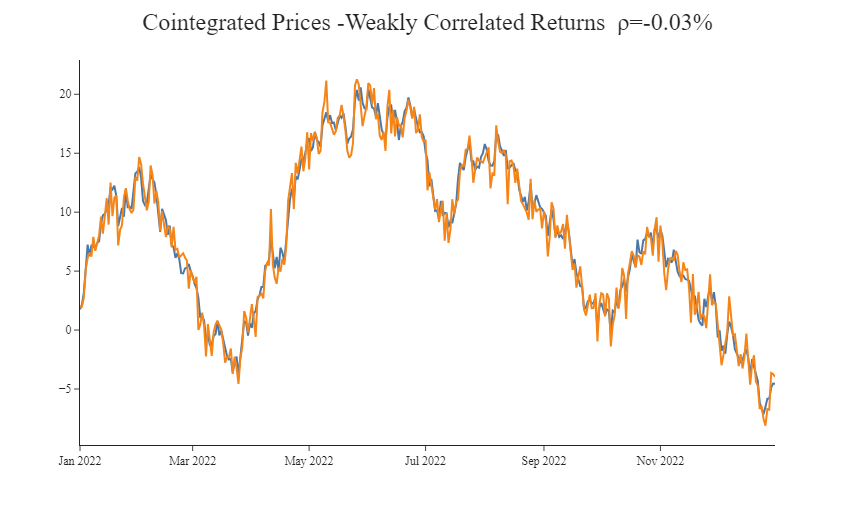
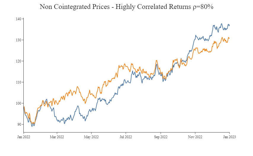
Cointegration vs Correlation

Cointegration and correlation are both statistical concepts used in the analysis of time series data, but they refer to different types of relationships between variables.

Correlation measures the strength and direction of a linear relationship between two variables. It tells us how much one variable tends to change when the other one does, but it doesn’t imply causation or a stable long-term relationship. Correlation is often represented by the Pearson correlation coefficient, which ranges from -1 (perfect negative correlation) to +1 (perfect positive correlation). A value of 0 indicates no correlation.

Cointegration, on the other hand, refers to a situation where two or more non-stationary time series are linked together in such a way that their linear combination is stationary. Even if the individual series themselves wander randomly over time, if they are cointegrated, there is a consistent, long-term equilibrium relationship between them. This concept is crucial in econometrics and finance as it suggests a predictable, long-term balance between the series, despite short-term fluctuations.

Example of Cointegration in Finance

1. Stock Indices and Tracking Portfolios:
   In the case of stock indices and tracking portfolios, consider the relationship between a major stock index like the S&P 500 and a mutual fund that aims to track its performance. Cointegration in this context would suggest that over the long term, the movements of the mutual fund are closely aligned with the movements of the S&P 500. Any short-term discrepancies between the fund and the index are expected to be temporary, with the fund consistently reflecting the performance of the index over an extended period.
2. Pairs Trading in Stocks:
   For pairs trading involving stocks, an example could be the shares of two major, competing corporations in the same industry, such as Coca-Cola and Pepsi. If these stocks are cointegrated, it indicates that while their individual stock prices might diverge due to short-term market factors, they exhibit a long-term parallel trend. This long-term relationship forms the basis of pairs trading strategies, where temporary price discrepancies between the stocks are seen as opportunities for arbitrage.
3. Spot and Futures Prices:
   In the realm of commodities, an example of cointegration can be observed between the spot and futures prices of a commodity, such as crude oil. Here, cointegration suggests a long-term equilibrium between the spot prices and futures prices of crude oil. Despite potential short-term divergences due to factors like storage costs or interest rates, these prices are expected to converge as the futures contract nears its expiration, reflecting their intrinsic linkage.
4. Commodities:
   When considering commodities like gold and silver, cointegration implies that their prices, though subject to individual market dynamics in the short term, share a long-term equilibrium relationship. This could be due to their similar market roles as precious metals and safe-haven assets, leading their prices to move in tandem over the long term despite short-term fluctuations.
5. Foreign Exchange:
   For foreign exchange, an example can be drawn from the cointegration between currency pairs like EUR/USD and GBP/USD. This cointegration would indicate that, over the long term, these currency pairs move together, maintaining a stable relationship. Short-term fluctuations may occur due to immediate economic events or policy changes, but the long-term movement reflects the enduring economic interrelations among the Eurozone, the UK, and the USA.
6. Economics:
   In an economic context, consider the Gross Domestic Product (GDP) and Consumer Price Index (CPI) of a country. Cointegration between these two indicators would imply that over a long period, the country’s economic growth (as measured by GDP) and inflation rate (as indicated by CPI) move in a correlated manner. While short-term deviations may arise from various economic policies or external factors, the long-term trend shows a consistent relationship between economic growth and inflation.

Cointegration on DAX30

After defining cointegration and providing several examples, this section presents a case study of cointegration analysis on the German stock market index, the DAX 30. Initially, we examine the cointegration of the index and individual stocks. Subsequently, we introduce two methodologies used for index tracking: one focused on minimizing tracking error variance, and the other based on cointegration.

To retrieve data, we utilize the Official EOD Python API library. Our process begins with gathering data for the index and its constituents dating back to January 2010. Information on the constituents is accessible through the use of the get_fundamentals_data function.

1. Use the “demo” API key to test our data from a limited set of tickers without registering: AAPL.US | TSLA.US | VTI.US | AMZN.US | BTC-USD | EUR-USD
Real-Time Data and all of the APIs (except Bulk) are included without API calls limitations with these tickers and the demo key.
2. Register to get your free API key (limited to 20 API calls per day) with access to: End-Of-Day Historical Data with only the past year for any ticker, and the List of tickers per Exchange.
3. To unlock your API key, we recommend to choose the subscription plan which covers your needs.

# get Dax30 data
start = "2010-01-01"
dax = api.get_historical_data("GDAXI.INDX", interval="d", iso8601_start=start,
iso8601_end="2024-01-09")["adjusted_close"].astype(float)
dax.name = "DAX"
# get constituents
comps = api.get_fundamentals_data("GDAXI.INDX")
comps = pd.DataFrame.from_dict(comps["Components"], orient="index")
# get times series data for Dax stocks
dax_comps_ts = pd.DataFrame()
for symbol in comps["Code"][:-4]:
    print(symbol)
    ts = api.get_historical_data("{}.XETRA".format(symbol), interval="d", iso8601_start=start,
                                 iso8601_end="2024-01-01")["adjusted_close"]
    ts.name = symbol
    dax_comps_ts = pd.concat([dax_comps_ts, ts], axis=1)

dax_comps_ts = dax_comps_ts.sort_index()
dax_comps_ts.index = pd.to_datetime(dax_comps_ts.index)
#merge the index and constituents data
df = pd.merge(dax, dax_comps_ts, 
                        left_on=dax.index, 
                        right_on=dax_comps_ts.index).set_index("key_0").astype(float)
df.index.name = "Date"

Next, we examine the dataset for missing values and remove those series that contribute the most to these gaps. This approach aids in creating a more extensive dataset, which is particularly beneficial in the context of regression analysis.

df = df.drop(columns= ["ZAL", "1COV", "VNA"], axis=1)
df = df.dropna()
logprice_all = np.log(df)[1:] 
ret_all = df.pct_change()[1:]

Finally we run the Engle-Granger test. In this case, we test for cointegration between each of the companies one-by-one and the index, by running the following regression and the checking for stationarity of residuals through the ADF test.

$$ ln(I_{t}) = \alpha + B_{k} ln(P_{kt}) + \epsilon $$

for each k, where is a Dax30 constituents.

X_all = ret_all.drop("DAX", axis=1)
t_stats = {}

for col in X_all.columns:
    X = X_all[col]
    y=logprice_all["DAX"]
    model = sm.OLS(y, X).fit()
    t_stats[col] =adf_test(model.resid)[0]

We plot the t-stats and critical values. Surprisingly, only two stocks – HEN3 and BRN – appear to be cointegrated at 5% significance level.

Application to Benchmark Tracking

In this paragraph we introduce two approaches for index tracking. The first is a cointegration-based method which regresses the index log price on the log prices of selected stocks over a calibration period. This log transformation ensures homogeneity and valid application of OLS in the presence of cointegration. The second, namely TEVM, method is the traditional OLS estimation where the index returns are regressed on the index stocks returns and by construction minimizes the tracking error.

In both cases, we employed calibration periods of from 2 years of data preceding the portfolio construction date. The initial portfolios based on cointegration tracking were established on March 7, 2012, and the most recent ones were created on December 29, 2023. To maintain their relevance and accuracy, all portfolios underwent rebalancing at intervals of every 10 trading days. The new rebalancing weights are based the new Ordinary Least Squares (OLS) coefficients, which were recalculated for each rolling calibration period in the cointegration regression analysis.

Cointegration

Let’s start with the cointegration approach describe above. In this case, we regress the index log prices, in this case, the Dax 30, on the price of the historical DAX constituents and test for stationarity of residuals with ADF check as prescribed by the Engle-Granger test.

Note that:
“the application of OLS to non-stationary dependent variables such as log(index) is only valid in the special case of a cointegration relationship. The residuals are stationary if, and only if, the log(index) and the tracking portfolio are cointegrated. Unless the residuals from the above regression are found to be stationary, the OLS coefficients will be inconsistent and further inference based on them will be invalid. Therefore, testing for cointegration is an essential step in constructing cointegration-based tracking portfolios.” Alexander and Dimitriu (2002)

""" Cointegration"""
dax_comps_tss = [] 
date = []
x = logprice_all.drop("DAX", axis=1)
window_size = 500
for i in range(0, len(ret_all) - window_size + 1,  10):
    
    # Extract the current rolling window
    X_window = x.iloc[i:i+window_size]
    y_window = logprice_all["DAX"].iloc[i:i+window_size]
    X_window = sm.add_constant(X_window)
    model = sm.OLS(y_window, X_window).fit()
    dax_comps_tss.append(model.params)
    date.append(X_window.index[-1])
    print(adf_test(model.resid)[0])
params = pd.DataFrame(dax_comps_tss, index=date)
params = params.drop("const", axis=1)
weights_coin = params.div(params.sum(axis=1), axis=0)

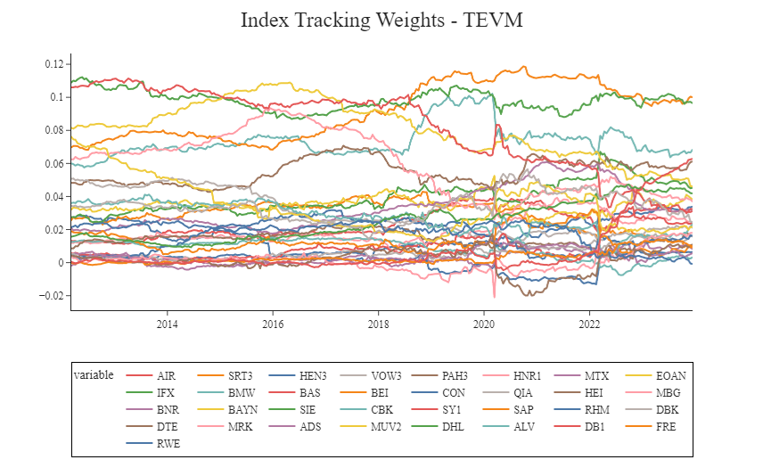
fig  = px.line(params)
fig.update_layout(title_text="Index Tracking Weights - Cointegration", xaxis_title="", yaxis_title="")
fig.show()

TEVM

Traditional benchmark tracking optimization problem is to minimize the tracking error with respect to the benchmark. This approach is also called TEVM. In this case, ordinary least squares is used to estimate a linear regression of benchmark returns against asset returns.

The calculated regression betas define the portfolio weights, with the residual representing the tracking error. However, this approach does not guarantee that the tracking error will exhibit mean-reversion characteristics.

Results and Conclusion

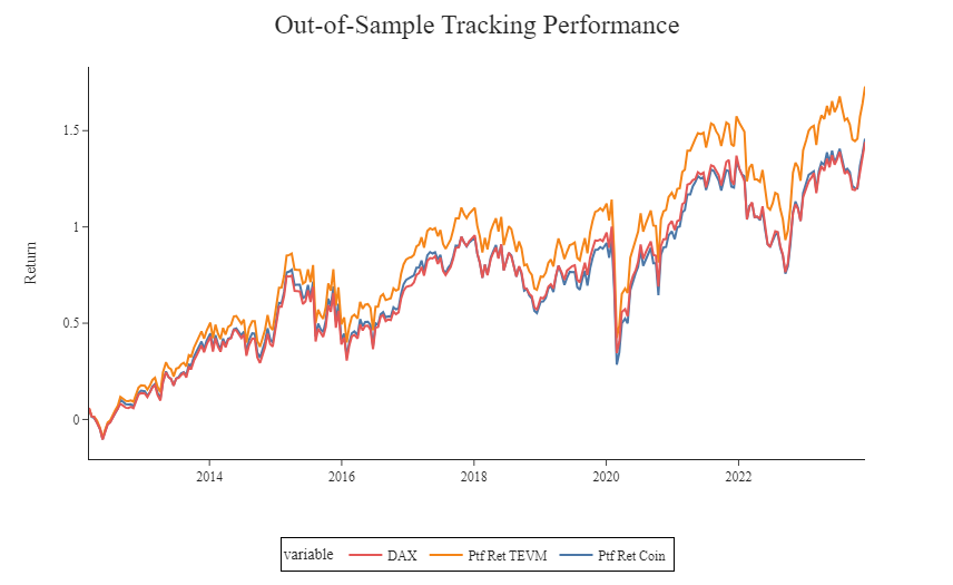
Finally we compare the results obtained with the two methods. As shown in the below figure, appropriate replicas can be constructed for the market index, provided that a minimum number of stocks is included in the tracking portfolio and an appropriate calibration period is used. Also it’s clear how the cointegration approach yields a better tracking performance compared to the variance minimization method.

In conclusion, this article presents a comprehensive study of cointegration and its application in the context of the German stock market, particularly focusing on the DAX 30 index. The application of the Engle-Granger test for cointegration between the DAX 30 and its constituents over the sample period revealed that only a few stocks demonstrated significant cointegration.

The exploration of index tracking methodologies, namely cointegration-based tracking and tracking error variance minimization (TEVM), highlighted the nuances and effectiveness of each approach. The cointegration-based method, which involves selecting stocks and determining portfolio holdings through cointegration optimization, has proven to be effective, especially when rebalanced regularly based on recalculated OLS coefficients. Our backtesting results underscore the efficacy of these methods in constructing market index replicas. Notably, the cointegration approach showed superior tracking performance compared to TEVM, underlining its potential in the realm of portfolio management.

Register & Get Data

Full code available here
Website: baglinifinance.com