
Time series analysis is a fundamental component of statistical studies and forecasting in various fields such as economics, finance, environmental science, and many more. In this comprehensive guide, we will delve into an example of time series analysis and show how to forecast economic variables with ARIMA model. In this case, we will use the Unemployment Rate in the United States and provide detailed insights and statistical formalization of each step in the process.
Quick jump:
Data Collection and Preprocessing
The journey begins with data collection, which is done through the Official EODHD APIs library. This is a important steps to step that enables the connection to an external data source to retrieve the data. For this case study, we retrieve US unemployment data from 1960. The snippet:
1. Use the “demo” API key to test our data from a limited set of tickers without registering: AAPL.US | TSLA.US | VTI.US | AMZN.US | BTC-USD | EUR-USD
Real-Time Data and all of the APIs (except Bulk) are included without API calls limitations with these tickers and the demo key.
2. Register to get your free API key (limited to 20 API calls per day) with access to: End-Of-Day Historical Data with only the past year for any ticker, and the List of tickers per Exchange.
3. To unlock your API key, we recommend to choose the subscription plan which covers your needs.
from utils.config import apikey
api = APIClient(apikey)

# Fetch and preprocess data
unemployment_data = pd.DataFrame(api.get_macro_indicators_data("USA", "unemployment_total_percent"))[["Date", "Value"]]
unemployment_data = unemployment_data.set_index("Date").sort_index()
unemployment_data.index = pd.to_datetime(unemployment_data.index)
unemployment_data = unemployment_data.asfreq(freq='A')
unemployment_data.head()
illustrates how data is fetched and transformed into a Pandas DataFrame for ease of manipulation.
Next, the data undergoes preprocessing. Timestamps are standardized, and the series is structured with an annual frequency. This structuring is vital for ensuring consistency in time intervals, a strict requirement in ARIMA models.
Also we split our data into a estimation and prediction sample. In our case, 90% of the data will be used to estimated the model coefficients while and the remaining 10% to check to quality of our forecast.
# Splitting the time series data
split_percentage = 0.9
split_index = int(len(unemployment_data) * split_percentage)
training_data = unemployment_data[:split_index]
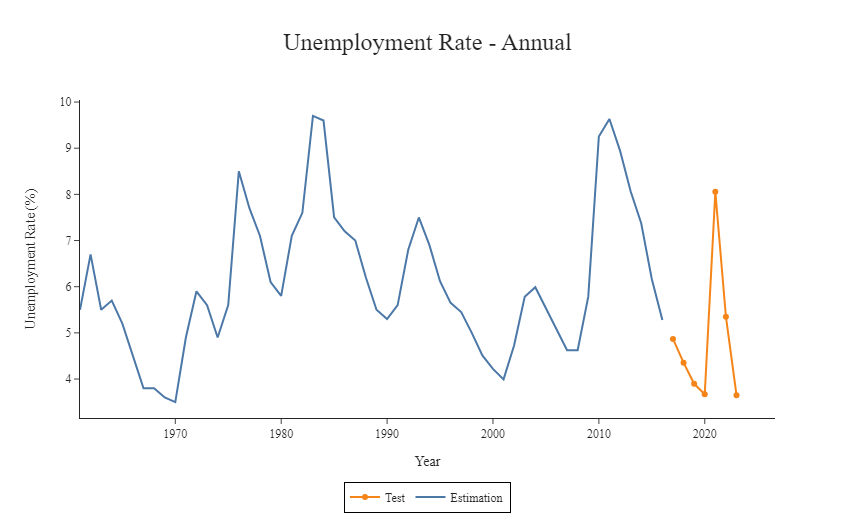
test_data = unemployment_data[split_index:]Finally we plot the whole time series for better visualization
Stationarity
A stationary process in time series analysis refers to a stochastic process whose statistical properties do not change over time. This implies that the process generates a series of data points where its mean, variance, and autocorrelation structure remain constant over time, irrespective of the period at which they are measured. This characteristic is essential because many statistical methods and models for time series analysis are based on the assumption of stationarity. Stationarity makes the series easier to analyze and predict, as the properties of the series do not change over time.
In practical terms, a stationary process can be visualized as a time series plot where the series fluctuates around a constant mean level, and the amplitude of the fluctuations does not increase or decrease over time. This consistency over time allows for the application of various time series forecasting methods, such as ARIMA (Auto-Regressive Integrated Moving Average) models, which assume that the series is stationary or has been transformed into a stationary series. In economics, individual time series are usually integrated processes, but sometimes the spread between two variables can be stationary and in this case we can say the prices are cointegrated.
Augmented Dickey-Fuller (ADF)
Generally, time series analysis commences with the Augmented Dickey-Fuller (ADF) test, which is a formal statistical test to check for stationarity. Here’s a short formalization of the test:

is the difference of the time series at time t
is a constant (intercept).
represents a deterministic time trend.
is the coefficient on the lagged level of the time series.
are the coefficients of the lagged differences of the series.
is the error term.
The null hypothesis H0 states that there is a unit root, implying the time series is non-stationary. Mathematically, this means 

# Function to perform the Augmented Dickey-Fuller test
def adf_test(time_series):
    result = adfuller(time_series)
    print('ADF Statistic: %f' % result[0])
    print('p-value: %f' % result[1])
    print('Critical Values:')
    for key, value in result[4].items():
        print('\t%s: %.3f' % (key, value))
    if result[1] > 0.05:
        print("Series is non-stationary")
    else:
        print("Series is stationary")

# Perform ADF test on the training data
adf_test(training_data['Value'])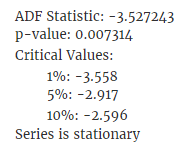
Once we have tested the stationarity of the process, we can move to the model fitting.
ARIMA Models
ARIMA (AutoRegressive Integrated Moving Average) is a widely used statistical method in time series forecasting. It combines autoregressive features (AR), integration (I – used for making the series stationary), and moving average (MA) components. The model is generally denoted as ARIMA(p, d, q), where:
- p (AR part): This represents the ‘autoregressive’ aspect of the model. It is the number of lag observations included in the model. Essentially, it is the degree to which current values of the series are dependent on its previous values.
- d (I part): The ‘integrated’ part, d, denotes the number of times the data needs differencing to make the time series stationary.
- q (MA part): The ‘moving average’ aspect. It is the size of the moving average window, indicating the number of lagged forecast errors that should go into the ARIMA model.
Formally, an ARIMA(p, d, q) model can be described as:

Here, L is the lag operator, 

The auto_arima function from the pmdarima library automates the process of selecting the best set of parameters (p, d, q) by iterating over multiple combinations and evaluating their performance.
# Building and fitting the ARIMA model
model_autoARIMA = auto_arima(training_data, start_p=0, start_q=0,
test='adf', max_p=2, max_q=2, m=1,
d=None, seasonal=False, start_P=0,
D=0, trace=True,
error_action='ignore',
suppress_warnings=True,
stepwise=True)
print(model_autoARIMA.summary())
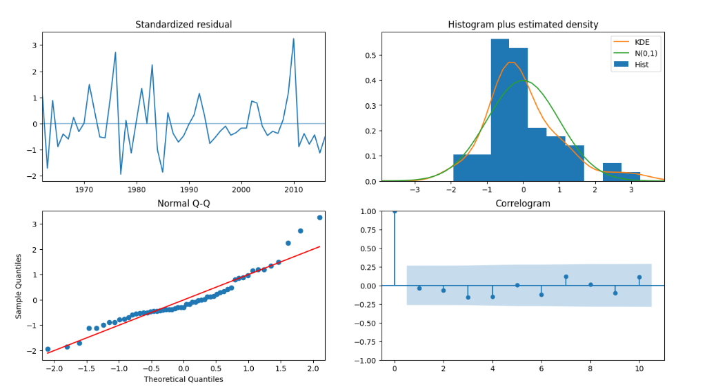
model_autoARIMA.plot_diagnostics(figsize=(15,8))
plt.show()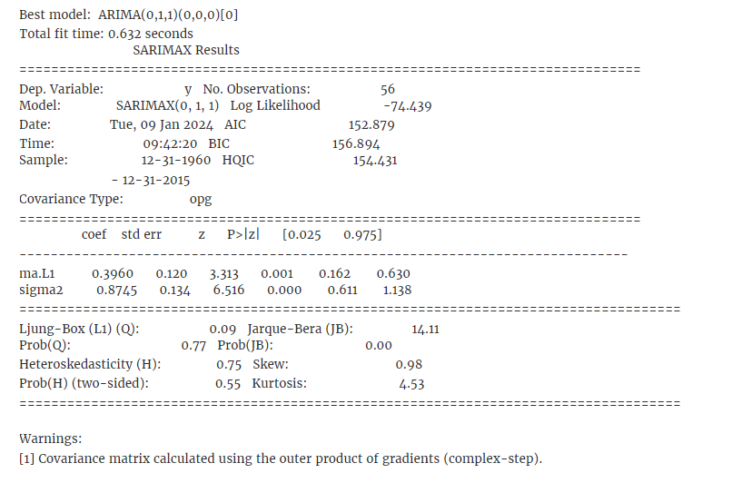
Looking at the results of the auto_arima function, it is evident how the combination I=1 and Q=1 is the one that best fits the current data. For this reason, we will now estimate the models parameters and derive forecasts using those arguments in the statsmodels.tsa.arima.model.ARIMA function.
# Fitting the ARIMA model
model = ARIMA(training_data, order=(0,1,1))
fitted_model = model.fit()
print(fitted_model.summary())
The final stage involves forecasting the unemployment rates using the fitted ARIMA model. The forecast is then compared against the actual data in the test set, using metrics like the Mean Squared Error (MSE) and Root Mean Squared Error (RMSE) to assess accuracy. The results are visually represented through plots showing the estimation data and forecasted values.
# Forecasting
forecast_steps = len(test_data)
forecast_results = fitted_model.get_forecast(steps=forecast_steps)
forecast_series = pd.Series(forecast_results.predicted_mean, index=test_data.index)

# Evaluating the forecast
mse = mean_squared_error(test_data, forecast_series)
rmse = mse**0.5

# Plotting the forecast results
plt.figure(figsize=(14,7))
plt.plot(training_data, label='Training Data')
plt.plot(test_data, label='Actual Data', color='orange')
plt.plot(forecast_series, label='Forecasted Data', color='green')
plt.fill_between(test_data.index,
                 forecast_results.conf_int().iloc[:, 0],
                 forecast_results.conf_int().iloc[:, 1],
                 color='k', alpha=.15)
plt.title('ARIMA Model Forecast Evaluation')
plt.xlabel('Year')
plt.ylabel('Unemployment Rate (%)')
plt.legend()
plt.show()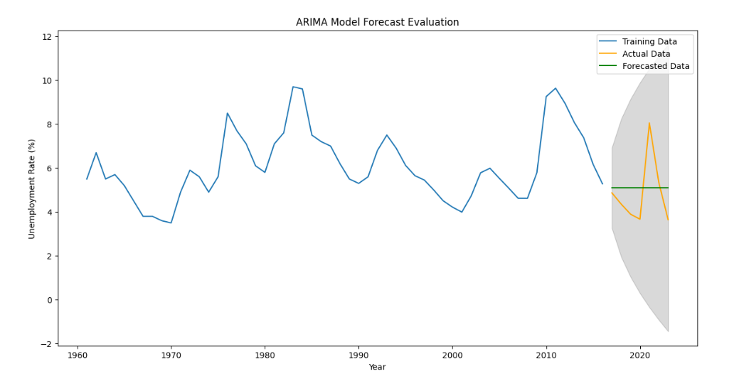
Conclusion
In this article, we introduced the concept of stationarity and showed a simple application of ARIMA model to forecast economic variables with ARIMA model. This comprehensive approach from data gathering, preprocessing, model building, to forecasting and evaluation exemplifies the intricate process of time series analysis using ARIMA models. It underscores the critical importance of understanding both the data and the underlying statistical methods for effective forecasting, particularly in areas as significant as economic indicators like unemployment rates.