S&P 500 – SMA200 Trading Strategy

Medium-to-Long term investing into the S&P 500

What is the S&P 500?

The S&P 500 was established in 1957, and is a stock market index that measures the stock performance of 500 large companies listed on stock exchanges in the United States. It is one of the most widely followed equity indices in the world and serves as an indicator and predictor of future trends or events for the U.S. stock market. The significant history of the S&P 500 is valuable for both real-world financial strategies and academic studies allowing for in-depth historical analysis. It is also great for backtesting trading strategies to evaluate how they perform in a variety of different conditions.

The S&P 500 represents approximately 80% of the total market value of the U.S. stock market. As such, it gives a good indication of the overall health and performance of the U.S. equity market. If you are interested in which companies are in the S&P 500, you can find the list of companies on Wikipedia. You may notice that there are in fact more than 500 entries in the S&P 500, and that is because some companies have more than one class of share.

The S&P 500 is also useful in that it covers a wide variety of sectors, making it more diversified than indices that track a specific sector. This diversity can provide a broader picture of the economic health across various industries.

The S&P 500 is used as a benchmark by many investment funds and portfolio managers to gauge the relative performance of their investments. When you hear that a fund “outperformed the S&P 500,” it means the fund did better than the average return of the 500 stocks in the index over the same period.

Many financial products, such as mutual funds and exchange-traded funds (ETFs), are tied to or based on the S&P 500. This makes it easier for individual investors to invest in a product that mirrors the performance of the broader market.

The wide media coverage of the S&P 500, coupled with the availability of derivative products (like futures and options), makes it popular among traders and investors.

Stocks that are part of the S&P 500 are among the most traded in the world, which means they are highly liquid. This liquidity is attractive to traders and large institutional investors because they can make large transactions without significantly affecting the stock price.

The performance of the S&P 500 is often used as a proxy for the overall U.S. economy’s health. Rising markets might suggest investor optimism about the economy, while declining markets can indicate pessimism.

S&P 500 Historical Data

You are able to obtain the historical data for the S&P 500 from EODHD API’s. The full documentation of their APIs can be found on their website. I personally prefer to use their official Python library and it vastly simplifies access to the data.

Register & Get Data

Using the Python library

The prerequisites for using the Python library is to have Python and PIP installed. There are plenty of guides available online, but I would recommend the Real Python documentation. If all has gone to plan you should be able to check the Python and PIP versions like this:

% python3 --version       
Python 3.11.4
% pip3 --version          
pip 23.2.1 from /usr/local/lib/python3.11/site-packages/pip (python 3.11)
% python3 -m pip --version
pip 23.2.1 from /usr/local/lib/python3.11/site-packages/pip (python 3.11)

You will also want to install the Python virtual environment (“venv”) as follows:

% python3 -m pip install virtualenv

% python3 -m venv --help   
usage: venv [-h] [--system-site-packages] [--symlinks | --copies] [--clear] [--upgrade] [--without-pip] [--prompt PROMPT] [--upgrade-deps] ENV_DIR [ENV_DIR ...]

Creates virtual Python environments in one or more target directories.

Presuming you have Python3, PIP3, and venv installed, the next step is to create yourself a working directory and virtual environment. Once that is done you will be able to install the Python library.

% mkdir EODHD_APIs
% cd EODHD_APIs
EODHD_APIs % python3 -m venv venv
EODHD_APIs % source venv/bin/activate
(venv) EODHD_APIs % python3 -m pip install eodhd -U
Collecting eodhd
Downloading eodhd-1.0.21-py3-none-any.whl (25 kB)
<snip>

Quick test to confirm the Python library installed properly

In order to confirm the “eodhd” Python library has installed correctly, we can run a quick test by creating a Python script and importing the library.

from eodhd import APIClient


def main():
    api = APIClient("<Your_API_Key>")
    print(isinstance(api, APIClient))


if __name__ == "__main__":
    main()

Running the script will look like this:

(venv) EODHD_APIs % python3 main.py 
Traceback (most recent call last):
  File "/EODHD_APIs/venv/lib/python3.11/site-packages/eodhd/apiclient.py", line 78, in __init__
    raise ValueError("API key is invalid")
ValueError: API key is invalid
(venv) EODHD_APIs %

The error is expected as I didn’t include my API key from EODHD APIs. If you don’t already have an API key, you will need to register for one.

The main objective of this test is to confirm the library imports and runs without an error, and it does.

Retrieving the S&P 500 data

I want to find the S&P 500 index on EODHD APIs, but I can’t remember the stock code. I’m going to show you how I located it.

The first step was to find the exchange code for “London Exchange”.

    df = api.get_exchanges()
    print(df[df["Name"].str.contains("London Exchange")])

I can see it’s “LSE“. I know the index I’m looking for is an ETF from HSBC.

    df = api.get_exchange_symbols("LSE")
    df = df[df["Type"] == "ETF"]
    df = df[df["Name"].str.contains("HSBC")]
    df = df[df["Name"].str.contains("500")]
    print(df)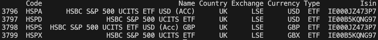

I can see it there, it’s “HSPX“.

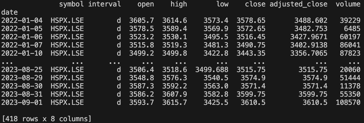
I now want to populate three data frames with Weekly, Daily and Hourly data.

    df_weekly = api.get_historical_data(symbol="HSPX.LSE", interval="w", iso8601_start="2018-01-01", iso8601_end="2023-09-04")
    print(df_weekly)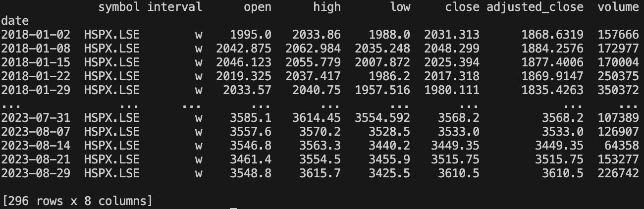

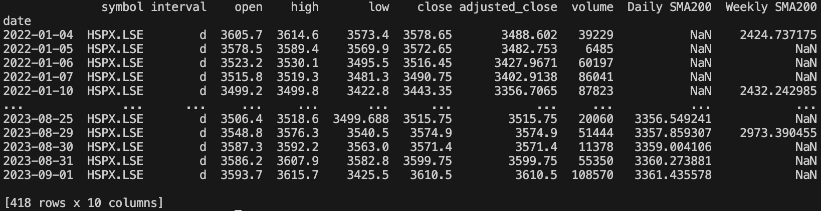
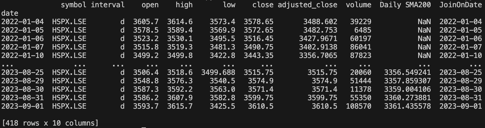
    df_daily = api.get_historical_data(symbol="HSPX.LSE", interval="d", iso8601_start="2022-01-01", iso8601_end="2023-09-04")
    print(df_daily)

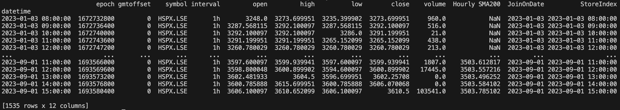
    df_hourly = api.get_historical_data(symbol="HSPX.LSE", interval="1h", iso8601_start="2023-01-01", iso8601_end="2023-09-04")
    print(df_hourly)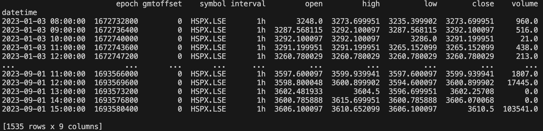

Calculating the 200-interval Simple Moving Averages (SMA)

It’s time to introduce the trading strategy…

What we want to do is calculate the SMA200 for the weekly, daily, and hourly. The first deciding factor is if the SMA200 for the daily is above or below the SMA200 for the weekly. If it’s above, then the long term trend is up and we want to be trading, and if it’s below the long term trend is down and we don’t want to be trading.

Assuming the SMA200 for the daily is above the SMA200 for the weekly, we then want to compare the SMA200 for the daily with the SMA200 for the hourly. If the SMA200 for the hourly crosses above the SMA200 for the daily, that’s a buy signal. If the SMA200 for the hourly crosses below the SMA200 for the daily, that’s a sell signal.

Now that we’ve covered the basics, let’s create our moving averages for the three datasets.

df_weekly["Weekly SMA200"] = df_weekly["adjusted_close"].rolling(200, min_periods=200).mean()

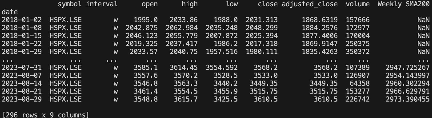
As you can see we now have a feature called “Weekly SMA200” which starts showing the mean of the previous 200 weeks. The NaN means “Not a Number” and just means that the first 200 weeks we don’t have a mean yet.

df_daily["Daily SMA200"] = df_daily["adjusted_close"].rolling(200, min_periods=200).mean()

df_hourly["Hourly SMA200"] = df_hourly["close"].rolling(200, min_periods=200).mean()

Merging the Daily and Weekly datasets

We will now want to start merging the three datasets for comparison. A copy of the daily dataset with the SMA200 will be created and the SMA200 for the weekly will be merged in.

    df_weekly_daily = df_daily.copy()
    df_weekly_daily["Weekly SMA200"] = df_weekly["Weekly SMA200"]
    print(df_weekly_daily)

To visualise this we can use the “plot” function in Pandas, which uses Matplotlib.

import matplotlib.pyplot as plt

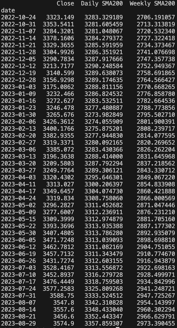
    df_plot = df_weekly_daily.dropna().loc["2022":"2023", ["adjusted_close", "Daily SMA200", "Weekly SMA200"]]
    df_plot.rename(columns={"adjusted_close": "Close"}, inplace=True)
    print(df_plot)
    df_plot.plot(title="S&P 500 Weekly SMA 200 vs. Daily SMA 200", kind="line", color=["black", "green", "blue"], figsize=(36, 12))
    plt.show()

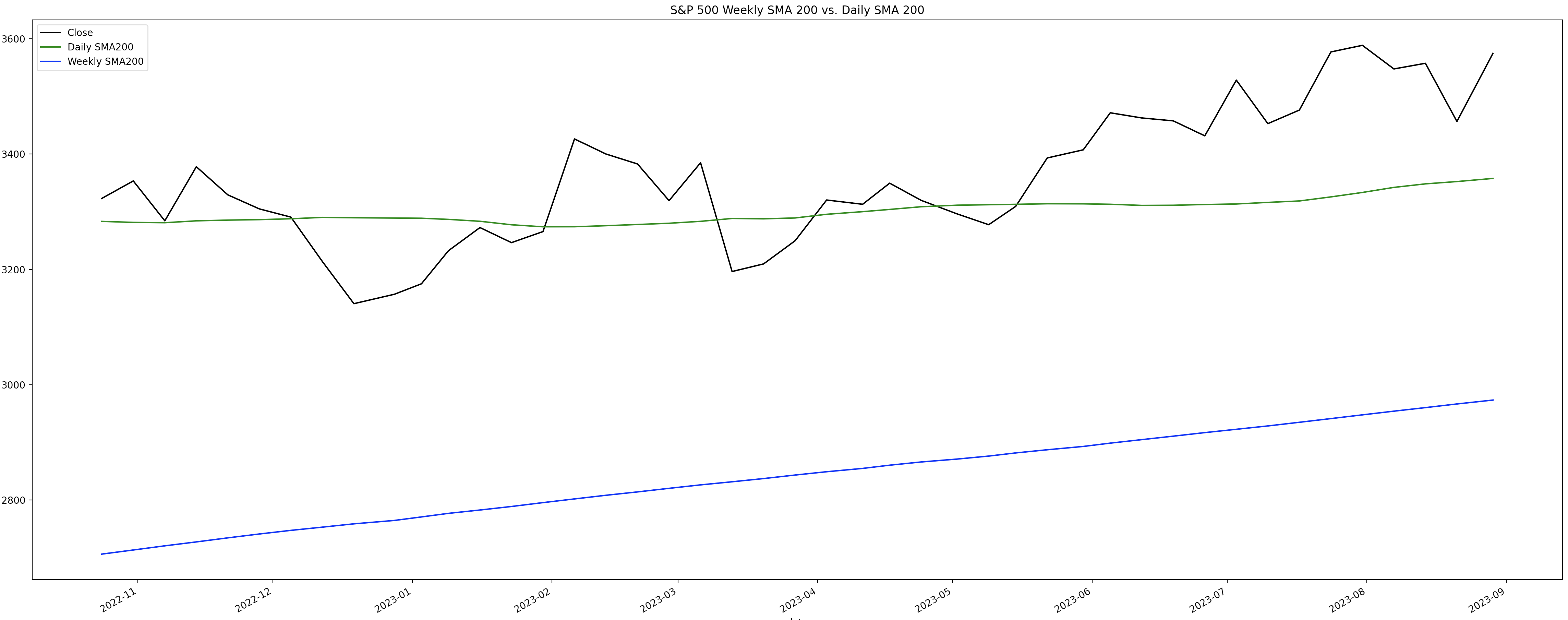
The blue line is the weekly SMA200, and as you can see is trending upwards which is good. More importantly the green line which is the daily SMA200 is way above the SMA200 for the weekly. This is a strong indication that the S&P 500 is a really good option to be trading.

Merging the Daily and Hourly datasets

The question now is when do we get in and out of our positions. To do this we’ll need to compare the SMA200 for the Daily and the SAM for the Hourly.

I want to merge the daily SMA200 dataframe with the hourly SMA200 dataframe. This is not as straightforward as it sounds. The index for the daily is only a date, but the index for the hourly is a date and time. This will prevent this from working without some work.

The way I resolved this is to create a new dataframe called, “df_hourly2” with a copy of the, “df_hourly” dataframe. I created a new feature called “JoinOnDate” with only the date from the date and time index. I also stored the current index for later in “StoreIndex”.

    df_hourly2 = df_hourly.copy()
    df_hourly2["JoinOnDate"] = df_hourly.index.date
    df_hourly2["JoinOnDate"] = pd.to_datetime(df_hourly2["JoinOnDate"]).dt.date
    df_hourly2["StoreIndex"] = df_hourly.index
    print(df_hourly2)

    df_daily2 = df_daily.copy()
    df_daily2["JoinOnDate"] = df_daily2.index
    df_daily2["JoinOnDate"] = pd.to_datetime(df_daily2["JoinOnDate"]).dt.date
    print(df_daily2)

    df_daily_hourly = df_hourly2.merge(df_daily2[["JoinOnDate", "Daily SMA200"]], on="JoinOnDate", how="left").set_index("StoreIndex")
    df_daily_hourly.index.name = "Date"
    df_daily_hourly.drop(["JoinOnDate"], axis=1, inplace=True)
    print(df_daily_hourly)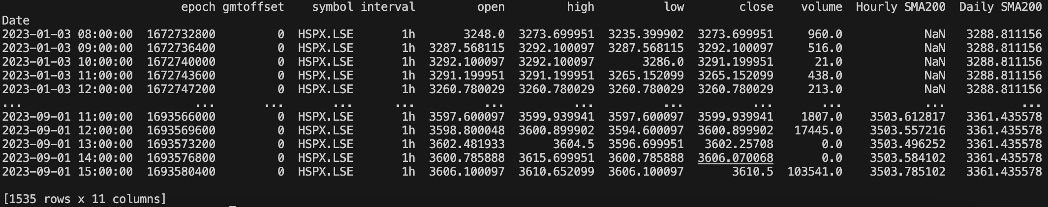

    df_plot = df_daily_hourly.dropna().loc["2023", ["close", "Daily SMA200", "Hourly SMA200"]]
    df_plot = df_plot[df_plot["close"] != 0]
    df_plot.rename(columns={"close": "Close"}, inplace=True)
    df_plot.plot(title="S&P 500 Weekly SMA 200 vs. Daily SMA 200", kind="line", color=["black", "green", "blue"], figsize=(36, 12))
    plt.show()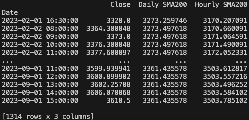

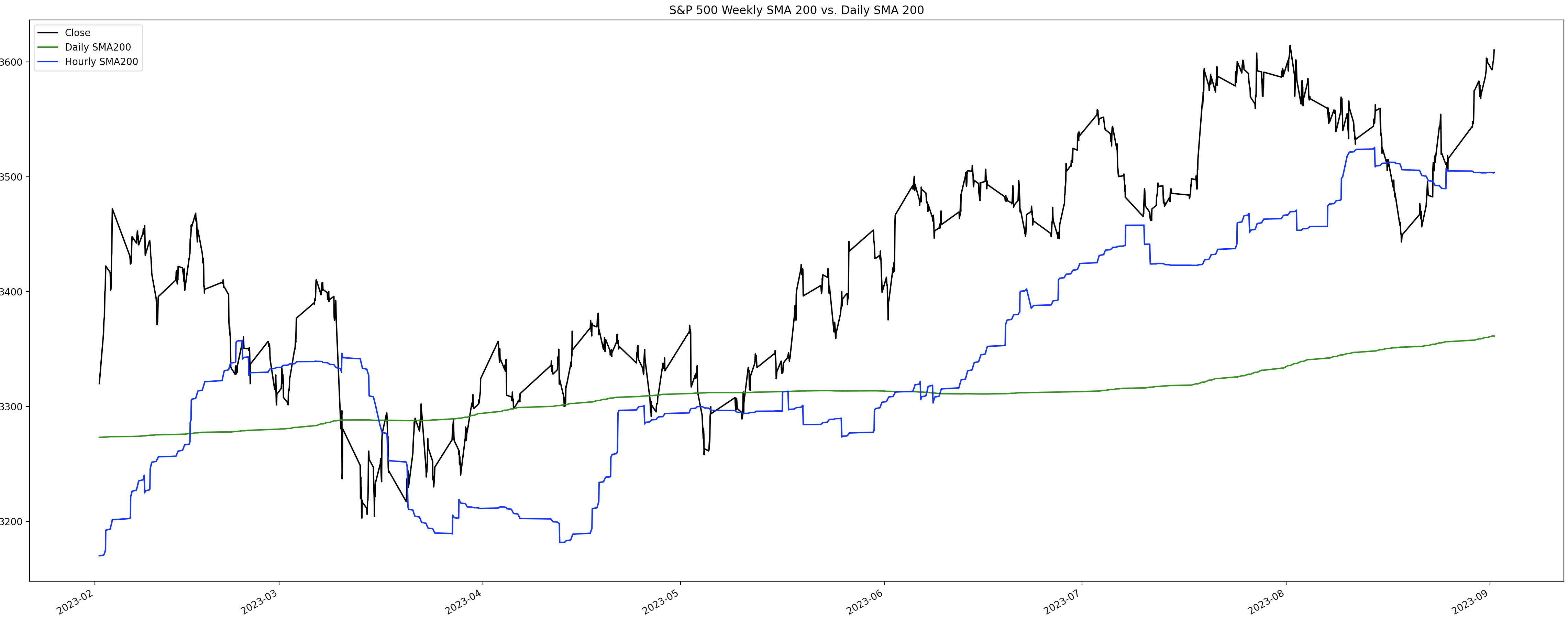
The blue line is the Hourly SMA200, and the green line is the Daily SMA200. As you can see the Hourly SMA200 is above the Daily SMA200 which is really good. You can also see visually when the Daily crossed above the Weekly SMA200 which resulted in a strong upward trend on the price. If you had bought mid-June 2023 when the crossover happened, you would be in a pretty decent position now.

In summary

Register & Get Data

Buy signal:

• Daily SMA200 > Weekly SMA200
• Hourly SMA200 > Daily SMA200

Sell signal:

• Hourly SMA200 < Daily SMA200

This strategy is not a day trading strategy. It’s meant for medium to long term investing. It’s tried and tested and confirmed with backtesting covering many years. A trade with some leverage would in almost all cases result in a profitable trade.

I know one person who has been using this for years and in the last 100 trades, he had a 99% success rate which is pretty outstanding. I’m not sure what would have happened in that one failed trade but I expect he didn’t wait until the Hourly SMA200 had cleanly crossed above the Daily SMA200.