

There are four different branches of technical indicators out there but the most popular ones are known as trend indicators. These indicators help traders in identifying the direction and strength of the market trend and trade along with them. In most cases, the indicators that come under the category of trend reveal good results unless we use them efficiently.
In this article, we are going to explore one of the most popular trend indicators, the Average Directional Index (shortly known as ADX). We will first build some basic understanding of what ADX is all about and its calculation, then, move on to building the indicator from scratch and construct a trading strategy based on that indicator in Python. To evaluate our strategy, we will first backtest it with the Apple stock, and then to make more sense, we will compare our strategy returns with the SPY ETF returns (an ETF specifically designed to track the movement of the S&P 500 index).
Quick jump:
- 1 Average True Range (ATR)
- 2 Average Directional Index (ADX)
- 3 Implementation in Python
- 3.1 Step-1: Importing Packages
- 3.2 Step-2: API Key Activation
- 3.3 Step-3: Extracting Historical Data
- 3.4 Step-4: ADX Calculation
- 3.5 Step-5: ADX Plot
- 3.6 Step-6: Creating the trading strategy
- 3.7 Step-7: Plotting the trading signals
- 3.8 Step-8: Creating our Position
- 3.9 Step-9: Backtesting
- 3.10 Step-10: SPY ETF Comparison
- 4 Final Thoughts!
Average True Range (ATR)
Before moving on to discovering ADX, it is essential to know what the Average True Range (ATR) is as it is involved in the calculation of the Average Directional Index (ADX).
The Average True Range is a technical indicator that measures how much an asset moves on an average. It is a lagging indicator meaning that it takes into account the historical data of an asset to measure the current value but it’s not capable of predicting the future data points. This is not considered as a drawback while using ATR as it’s one of the indicators to track the volatility of a market more accurately. Along with being a lagging indicator, ATR is also a non-directional indicator meaning that the movement of ATR is inversely proportional to the actual movement of the market. To calculate ATR, it is requisite to follow two steps:
- Calculate True Range (TR): A True Range of an asset is calculated by taking the greatest values of three price differences which are: market high minus market low, market high minus previous market close, and previous market close minus market low. It can be represented as follows:
MAX [ {HIGH - LOW}, {HIGH - P.CLOSE}, {P.CLOSE - LOW} ]

where,
MAX = Maximum values
HIGH = Market High
LOW = Market Low
P.CLOSE = Previous market close
- Calculate ATR: The calculation for the Average True Range is simple. We just have to take a smoothed average of the previously calculated True Range values for a specified number of periods. The smoothed average is not just any SMA or EMA but an own type of smoothed average created by Wilder Wiles himself but there aren’t any restrictions in using other MAs too. In this article, we will be using SMA to calculate ATR rather than the custom moving average created by the founder of the indicator just to make things simple. The calculation of ATR with a traditional setting of 14 as the number of periods can be represented as follows:
ATR 14 = EMA 14 [ TR ]

where,
ATR 14 = 14 Period Average True Range
SMA 14 = 14 Period Simple Moving Average
TR = True Range
While using ATR as an indicator for trading purposes, traders must ensure that they are cautious than ever as the indicator is very lagging. Now that we have an understanding of what the Average True Range is all about. Let’s now dive into the main concept of this article, the Average Directional Index.
Average Directional Index (ADX)
ADX is a technical indicator that is widely used in measuring the strength of the market trend. Now, the ADX doesn’t measure the direction of the trend, whether it’s bullish or bearish, but just represents how strong the trend is. So, to identify the direction of the trend, ADX is combined with a Positive Directional Index (+ DI) and a Negative Directional Index (- DI). As the name suggests, the + DI measures the bullish or positive trend of the market, similarly, the – DI measures the bearish or negative trend of the market. The values of all the components are bound between 0 to 100, hence acting as an oscillator. The traditional setting of ADX is 14 as the lookback period.
To calculate the values of ADX with 14 as the lookback period, first, the Positive (+ DM) and Negative Directional Movement (- DM) is determined. The + DM is calculated by finding the difference between the current high and the previous high, and similarly, the – DM is calculated by finding the difference between the previous low and the current low. It can be represented as follows:
+ DM = CURRENT HIGH - PREVIOUS HIGH
- DM = PREVIOUS LOW - CURRENT LOW
Then, an ATR with 14 as the lookback period is calculated. Now, using the calculated directional movement and the ATR values, the Positive Directional Index (+ DI) and the Negative Directional Index (- DI) are calculated. To determine the values of + DI, the value received by taking the Exponential Moving Average (EMA) of the Positive Directional Movement (+ DM) with 14 as the lookback period is divided by the previously calculated 14-day ATR and then, multiplied by 100. This same applies to determining the – DI too but instead of taking the 14-day EMA of + DM, the Negative Directional Movement (- DM) is taken into account. The formula to calculate both the + DI and the – DI can be represented as follows:
+ DI14 = 100 * [ EMA 14 ( + DM ) / ATR 14 ]
- DI14 = 100 * [ EMA 14 ( - DM ) / ATR 14 ]
The next step is to use the + DI and – DI to calculate the Directional Index. It can be determined by dividing the absolute value of the difference between the +DI and – DI by the absolute value of the total of + DI and – DI multiped by 100. The formula to calculate the Directional Index can be represented as follows:
DI 14 = | (+ DI 14) - (- DI 14) | / | (+ DI 14) + (- DI 14) | * 100
The final step is to calculate the ADX itself by utilizing the determined Directional Index values. The ADX is calculated by multiplying the previous Directional Index value with 13 (lookback period – 1) and adding it with the Directional Index, then multiplied by 100. The formula to calculate the values of ADX can be represented as follows:
ADX 14 = [ ( PREV DI 14 * 13 ) + DI 14 ] * 100
The ADX cannot be used as it is but needs to be smoothed. Since founded by Wilder Wiles (the founder of ATR too), the ADX is smoothed by a custom moving average we discussed before. We neglected using this custom moving average while calculating ATR as it is possible to use other types of moving averages but it is essential to use while smoothing ADX to get accurate values.
That’s the whole process of calculating the values of ADX. Now, let’s discuss how a simple ADX-based trading strategy can be constructed.
About our trading strategy
In this article, we are going to build a simple crossover strategy that reveals a buy signal whenever the ADX line crosses from below to above 25 and the + DI line is above the – DI line. Similarly, a sell signal is generated whenever the ADX line crosses from below to above 25 and the – DI line is above the + DI line. Our trading strategy can be represented as follows:
IF P.ADX < 25 AND C.ADX > 25 AND + DI LINE > - DI LINE ==> BUY
IF P.ADX < 25 AND C.ADX > 25 AND + DI LINE < - DI LINE ==> SELL
This concludes the theory part of this article. Now, let’s code this indicator from scratch and build the discussed trading strategy out of it in python and backtest it with the Apple stock to see some exciting results. We will also compare our ADX crossover strategy returns with the returns of the SPY ETF to see how well our trading strategy has performed against a benchmark. Without further ado, let’s dive into the coding part.
Implementation in Python
The coding part is classified into various steps as follows:
1. Importing Packages
2. API Key Activation
3. Extracting Historical Stock Data
4. ADX Calculation
5. ADX Indicator Plot
6. Creating the Trading Strategy
7. Plotting the Trading Lists
8. Creating our Position
9. Backtesting
10. SPY ETF Comparison
We will be following the order mentioned in the above list and buckle up your seat belts to follow every upcoming coding part.
Step-1: Importing Packages
Importing the required packages into the Python environment is a non-skippable step. The primary packages are going to be eodhd for extracting historical stock data, Pandas for data formatting and manipulations, NumPy to work with arrays and for complex functions, and Matplotlib for plotting purposes. The secondary packages are going to be Math for mathematical functions and Termcolor for font customization (optional).
Python Implementation:
# IMPORTING PACKAGES

import numpy as np
import matplotlib.pyplot as plt
import pandas as pd
from termcolor import colored as cl
from math import floor
from eodhd import APIClient

plt.rcParams['figure.figsize'] = (20,10)
plt.style.use('fivethirtyeight')
With the required packages imported into Python, we can proceed to fetch historical data for Apple using EODHD’s eodhd Python library. Also, if you haven’t installed any of the imported packages, make sure to do so using the pip command in your terminal.
Step-2: API Key Activation
It is essential to register the EODHD API key with the package in order to use its functions. If you don’t have an EODHD API key, firstly, head over to their website, then, finish the registration process to create an EODHD account, and finally, navigate to the ‘Settings’ page where you could find your secret EODHD API key. It is important to ensure that this secret API key is not revealed to anyone. You can activate the API key by following this code:
api_key = '<YOUR API KEY>'
client = APIClient(api_key)
The code is pretty simple. In the first line, we are storing the secret EODHD API key into the api_key and then in the second line, we are using the APIClient class provided by the eodhd package to activate the API key and stored the response in the client variable.
Note that you need to replace <YOUR API KEY> with your secret EODHD API key. Apart from directly storing the API key with text, there are other ways for better security such as utilizing environmental variables, and so on.
Step-3: Extracting Historical Data
Before heading into the extraction part, it is first essential to have some background about historical or end-of-day data. In a nutshell, historical data consists of information accumulated over a period of time. It helps in identifying patterns and trends in the data. It also assists in studying market behavior. Now, you can easily extract the historical data of any tradeable assets using the eod package by following this code:
# EXTRACTING HISTORICAL DATA

def get_historical_data(ticker, start_date):
    json_resp = client.get_eod_historical_stock_market_data(symbol = ticker, period = 'd', from_date = start_date, order = 'a')
    df = pd.DataFrame(json_resp)
    df = df.set_index('date')
    df.index = pd.to_datetime(df.index)
    return df

aapl = get_historical_data('AAPL', '2020-01-01')
aapl.tail()
In the above code, we are using the get_eod_historical_stock_market_data function provided by the eodhd package to extract the split-adjusted historical stock data of Apple. The function consists of the following parameters:
- the
tickerparameter where the symbol of the stock we are interested in extracting the data should be mentioned - the
periodrefers to the time interval between each data point (one-day interval in our case). - the
from_dateandto_dateparameters which indicate the starting and ending date of the data respectively. The format of the input should be “YYYY-MM-DD” - the
orderparameter which is an optional parameter that can be used to order the dataframe either in ascending (a) or descending (d). It is ordered based on the dates.
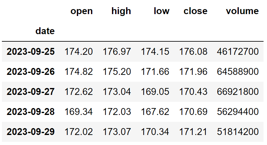
After extracting the historical data, we are performing some data-wrangling processes to clean and format the data. The final dataframe looks like this:
Step-4: ADX Calculation
In this step, we are going to calculate the values of ADX by following the method we discussed before.
Python Implementation:
def get_adx(high, low, close, lookback):
    plus_dm = high.diff()
    minus_dm = low.diff()
    plus_dm[plus_dm < 0] = 0
    minus_dm[minus_dm > 0] = 0

    tr1 = pd.DataFrame(high - low)
    tr2 = pd.DataFrame(abs(high - close.shift(1)))
    tr3 = pd.DataFrame(abs(low - close.shift(1)))
    frames = [tr1, tr2, tr3]
    tr = pd.concat(frames, axis = 1, join = 'inner').max(axis = 1)
    atr = tr.rolling(lookback).mean()

    plus_di = 100 * (plus_dm.ewm(alpha = 1/lookback).mean() / atr)
    minus_di = abs(100 * (minus_dm.ewm(alpha = 1/lookback).mean() / atr))
    dx = (abs(plus_di - minus_di) / abs(plus_di + minus_di)) * 100
    adx = ((dx.shift(1) * (lookback - 1)) + dx) / lookback
    adx_smooth = adx.ewm(alpha = 1/lookback).mean()
    return plus_di, minus_di, adx_smooth

aapl['plus_di'] = pd.DataFrame(get_adx(aapl['high'], aapl['low'], aapl['close'], 14)[0]).rename(columns = {0:'plus_di'})
aapl['minus_di'] = pd.DataFrame(get_adx(aapl['high'], aapl['low'], aapl['close'], 14)[1]).rename(columns = {0:'minus_di'})
aapl['adx'] = pd.DataFrame(get_adx(aapl['high'], aapl['low'], aapl['close'], 14)[2]).rename(columns = {0:'adx'})
aapl = aapl.dropna()
aapl.tail()
Output:
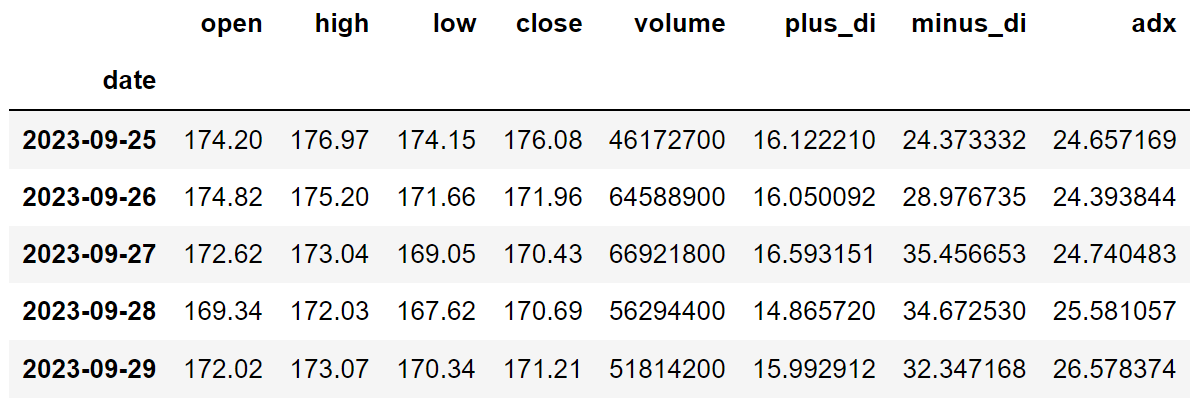
Code Explanation: We are first defining a function named ‘get_adx’ that takes a stock’s high (‘high’), low (‘low’), and close data (‘close’) along with the lookback period (‘lookback’) as parameters.
Inside the function, we are first calculating and storing the + DM and – DM into the ‘plus_dm’ and ‘minus_dm’ respectively. Then comes the ATR calculation where we are first calculating the three differences and defined a variable ‘tr’ to store the highest values among the determined differences, then, we calculated and stored the values of ATR into the ‘atr’ variable.
Using the calculated directional movements and ATR values, we are calculating the + DI and – DI and stored them into the ‘plus_di’ and ‘minus_di’ variables respectively. With the help of the previously discussed formula, we are calculating the Directional Index values and stored them into the ‘dx’ variable, and applied those values into the ADX formula to calculate the Average Directional Index values. Then, we defined a variable ‘adx_smooth’ to store the smoothed values of ADX. Finally, we are returning and calling the function to obtain the + DI, – DI, and ADX values of Apple with 14 as the lookback period.
Step-5: ADX Plot
In this step, we are going to plot the calculated ADX values of Apple to make more sense out of it. The main aim of this part is not on the coding section but instead to observe the plot to gain a solid understanding of the Average Directional Index.
Python Implementation:
ax1 = plt.subplot2grid((11,1), (0,0), rowspan = 5, colspan = 1)
ax2 = plt.subplot2grid((11,1), (6,0), rowspan = 5, colspan = 1)
ax1.plot(aapl['close'], linewidth = 2, color = '#ff9800')
ax1.set_title('AAPL CLOSING PRICE')
ax2.plot(aapl['plus_di'], color = '#26a69a', label = '+ DI 14', linewidth = 3, alpha = 0.3)
ax2.plot(aapl['minus_di'], color = '#f44336', label = '- DI 14', linewidth = 3, alpha = 0.3)
ax2.plot(aapl['adx'], color = '#2196f3', label = 'ADX 14', linewidth = 3)
ax2.axhline(25, color = 'grey', linewidth = 2, linestyle = '--')
ax2.legend()
ax2.set_title('AAPL ADX 14')
plt.show()
Output:
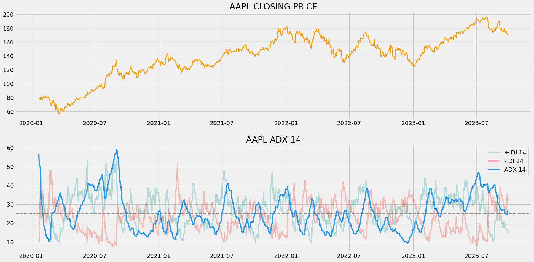
The above chart is divided into two panels: the upper panel with the closing prices of Apple and the lower panel with the components of ADX. Along with the components, a grey dashed line is plotted which is the threshold for the ADX plotted at a level of 25. As I said before, the ADX doesn’t track the direction of the trend but instead, the strength and it can be seen several times in the chart where the ADX line increases when the market shows a strong trend (either up or down) and decreases when the market bound to consolidate. This is the same case with both the directional index lines too. We could see that the + DI line increases when the market shows a sturdy uptrend and decreases during a downtrend and vice-versa for the – DI line.
ADX is not only used to quantify the strength of a market trend but also becomes a handy tool to identify ranging markets (markets where the stock moves back and forth between specific high and low levels showing zero momentum). Whenever the lines move closer to each other, the market is observed to be ranging, similarly, the wider the space between the lines, the more the markets are trending. Those who are introduced to the chart of ADX for the very first time might confuse themselves since the movement of each line is indirectly proportional to the movement of the market.
Step-6: Creating the trading strategy
In this step, we are going to implement the discussed Average Directional Index trading strategy in Python.
Python Implementation:
def implement_adx_strategy(prices, pdi, ndi, adx):
    buy_price = []
    sell_price = []
    adx_signal = []
    signal = 0

    for i in range(len(prices)):
        if adx[i-1] < 25 and adx[i] > 25 and pdi[i] > ndi[i]:
            if signal != 1:
                buy_price.append(prices[i])
                sell_price.append(np.nan)
                signal = 1
                adx_signal.append(signal)
            else:
                buy_price.append(np.nan)
                sell_price.append(np.nan)
                adx_signal.append(0)
        elif adx[i-1] < 25 and adx[i] > 25 and ndi[i] > pdi[i]:
            if signal != -1:
                buy_price.append(np.nan)
                sell_price.append(prices[i])
                signal = -1
                adx_signal.append(signal)
            else:
                buy_price.append(np.nan)
                sell_price.append(np.nan)
                adx_signal.append(0)
        else:
            buy_price.append(np.nan)
            sell_price.append(np.nan)
            adx_signal.append(0)

    return buy_price, sell_price, adx_signal

buy_price, sell_price, adx_signal = implement_adx_strategy(aapl['close'], aapl['plus_di'], aapl['minus_di'], aapl['adx'])
Code Explanation: First, we are defining a function named ‘implement_adx_strategy’ which takes the stock prices (‘prices), and the components of ADX (‘pdi’, ‘ndi’, ‘adx’) as parameters.
Inside the function, we are creating three empty lists (buy_price, sell_price, and adx_signal) in which the values will be appended while creating the trading strategy.
After that, we are implementing the trading strategy through a for-loop. Inside the for-loop, we are passing certain conditions, and if the conditions are satisfied, the respective values will be appended to the empty lists. If the condition to buy the stock gets satisfied, the buying price will be appended to the ‘buy_price’ list, and the signal value will be appended as 1 representing to buy the stock. Similarly, if the condition to sell the stock gets satisfied, the selling price will be appended to the ‘sell_price’ list, and the signal value will be appended as -1 representing to sell the stock.
Finally, we are returning the lists appended with values. Then, we are calling the created function and stored the values into their respective variables. The list doesn’t make any sense unless we plot the values. So, let’s plot the values of the created trading lists.
Step-7: Plotting the trading signals
In this step, we are going to plot the created trading lists to make sense out of them.
Python Implementation:
ax1 = plt.subplot2grid((11,1), (0,0), rowspan = 5, colspan = 1)
ax2 = plt.subplot2grid((11,1), (6,0), rowspan = 5, colspan = 1)
ax1.plot(aapl['close'], linewidth = 3, color = '#ff9800', alpha = 0.6)
ax1.set_title('AAPL CLOSING PRICE')
ax1.plot(aapl.index, buy_price, marker = '^', color = '#26a69a', markersize = 14, linewidth = 0, label = 'BUY SIGNAL')
ax1.plot(aapl.index, sell_price, marker = 'v', color = '#f44336', markersize = 14, linewidth = 0, label = 'SELL SIGNAL')
ax2.plot(aapl['plus_di'], color = '#26a69a', label = '+ DI 14', linewidth = 3, alpha = 0.3)
ax2.plot(aapl['minus_di'], color = '#f44336', label = '- DI 14', linewidth = 3, alpha = 0.3)
ax2.plot(aapl['adx'], color = '#2196f3', label = 'ADX 14', linewidth = 3)
ax2.axhline(25, color = 'grey', linewidth = 2, linestyle = '--')
ax2.legend()
ax2.set_title('AAPL ADX 14')
plt.show()
Output:
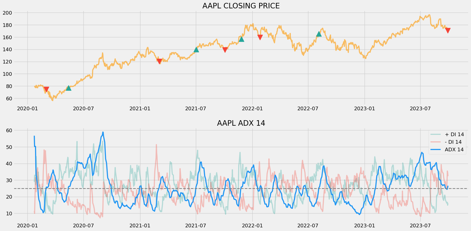
Code Explanation: We are plotting the Average Directional Index components along with the buy and sell signals generated by the trading strategy. We can observe that whenever the ADX line crosses from below to above 25 and the + DI line is above the – DI line, a green-colored buy signal is plotted in the chart. Similarly, whenever the ADX line crosses from below to above 25 and the + DI line is below the – DI line, a red-colored sell signal is plotted in the chart.
Step-8: Creating our Position
In this step, we are going to create a list that indicates 1 if we hold the stock or 0 if we don’t own or hold the stock.
Python Implementation:
position = []
for i in range(len(adx_signal)):
    if adx_signal[i] > 1:
        position.append(0)
    else:
        position.append(1)

for i in range(len(aapl['close'])):
    if adx_signal[i] == 1:
        position[i] = 1
    elif adx_signal[i] == -1:
        position[i] = 0
    else:
        position[i] = position[i-1]

close_price = aapl['close']
plus_di = aapl['plus_di']
minus_di = aapl['minus_di']
adx = aapl['adx']
adx_signal = pd.DataFrame(adx_signal).rename(columns = {0:'adx_signal'}).set_index(aapl.index)
position = pd.DataFrame(position).rename(columns = {0:'adx_position'}).set_index(aapl.index)

frames = [close_price, plus_di, minus_di, adx, adx_signal, position]
strategy = pd.concat(frames, join = 'inner', axis = 1)

strategy
Output:
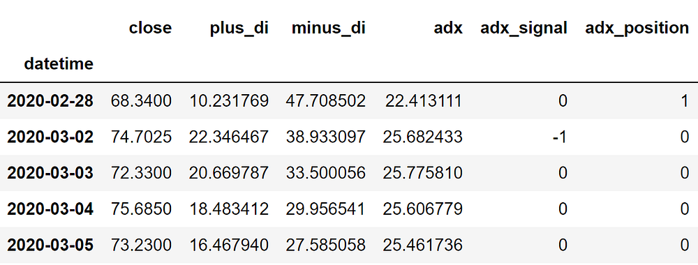
Code Explanation: First, we are creating an empty list named ‘position’. We are passing two for-loops, one is to generate values for the ‘position’ list to just match the length of the ‘signal’ list. The other for-loop is the one we are using to generate actual position values. Inside the second for-loop, we are iterating over the values of the ‘signal’ list, and the values of the ‘position’ list get appended concerning which condition gets satisfied. The value of the position remains 1 if we hold the stock or remains 0 if we sold or don’t own the stock. Finally, we are doing some data manipulations to combine all the created lists into one dataframe.
From the output being shown, we can see that in the first row our position in the stock has remained 1 (since there isn’t any change in the ADX signal) but our position suddenly turned to -1 as we sold the stock when the ADX trading signal represents a sell signal (-1). Our position will remain 0 until some changes in the trading signal occur. Now it’s time to do implement some backtesting process!
Step-9: Backtesting
Before moving on, it is essential to know what backtesting is. Backtesting is the process of seeing how well our trading strategy has performed on the given stock data. In our case, we are going to implement a backtesting process for our Average Directional Index trading strategy over the Apple stock data.
Python Implementation:
aapl_ret = pd.DataFrame(np.diff(aapl['close'])).rename(columns = {0:'returns'})
adx_strategy_ret = []

for i in range(len(aapl_ret)):
    returns = aapl_ret['returns'][i]*strategy['adx_position'][i]
    adx_strategy_ret.append(returns)

adx_strategy_ret_df = pd.DataFrame(adx_strategy_ret).rename(columns = {0:'adx_returns'})
investment_value = 100000
adx_investment_ret = []

for i in range(len(adx_strategy_ret_df['adx_returns'])):
    number_of_stocks = floor(investment_value/aapl['close'][i])
    returns = number_of_stocks*adx_strategy_ret_df['adx_returns'][i]
    adx_investment_ret.append(returns)

adx_investment_ret_df = pd.DataFrame(adx_investment_ret).rename(columns = {0:'investment_returns'})
total_investment_ret = round(sum(adx_investment_ret_df['investment_returns']), 2)
profit_percentage = floor((total_investment_ret/investment_value)*100)
print(cl('Profit gained from the ADX strategy by investing $100k in AAPL : {}'.format(total_investment_ret), attrs = ['bold']))
print(cl('Profit percentage of the ADX strategy : {}%'.format(profit_percentage), attrs = ['bold']))
Output:
Profit gained from the ADX strategy by investing $100k in AAPL : 54719.46
Profit percentage of the ADX strategy : 54%
Code Explanation: First, we are calculating the returns of the Apple stock using the ‘diff’ function provided by the NumPy package and we have stored it as a dataframe into the ‘aapl_ret’ variable. Next, we are passing a for-loop to iterate over the values of the ‘aapl_ret’ variable to calculate the returns we gained from our ADX trading strategy, and these returns values are appended to the ‘adx_strategy_ret’ list. Next, we are converting the ‘adx_strategy_ret’ list into a dataframe and stored it into the ‘adx_strategy_ret_df’ variable.
Next comes the backtesting process. We are going to backtest our strategy by investing a hundred thousand USD into our trading strategy. So first, we are storing the amount of investment into the ‘investment_value’ variable. After that, we are calculating the number of Apple stocks we can buy using the investment amount. You can notice that I’ve used the ‘floor’ function provided by the Math package because, while dividing the investment amount by the closing price of Apple stock, it spits out an output with decimal numbers. The number of stocks should be an integer but not a decimal number. Using the ‘floor’ function, we can cut out the decimals. Remember that the ‘floor’ function is way more complex than the ‘round’ function. Then, we are passing a for-loop to find the investment returns followed by some data manipulation tasks.
Finally, we are printing the total return we got by investing a hundred thousand into our trading strategy and it is revealed that we have made an approximate profit of fifty-four thousand USD in three years. That’s not bad! Now, let’s compare our returns with SPY ETF (an ETF designed to track the S&P 500 stock market index) returns.
Step-10: SPY ETF Comparison
This step is optional but it is highly recommended as we can get an idea of how well our trading strategy performs against a benchmark (SPY ETF). In this step, we are going to extract the data of the SPY ETF using the ‘get_historical_data’ function we created and compare the returns we get from the SPY ETF with our Average Directional Index strategy returns on Apple.
def get_benchmark(start_date, investment_value):
    spy = get_historical_data('SPY', start_date)['close']
    benchmark = pd.DataFrame(np.diff(spy)).rename(columns = {0:'benchmark_returns'})

    investment_value = investment_value
    benchmark_investment_ret = []

    for i in range(len(benchmark['benchmark_returns'])):
        number_of_stocks = floor(investment_value/spy[i])
        returns = number_of_stocks*benchmark['benchmark_returns'][i]
        benchmark_investment_ret.append(returns)

    benchmark_investment_ret_df = pd.DataFrame(benchmark_investment_ret).rename(columns = {0:'investment_returns'})
    return benchmark_investment_ret_df

benchmark = get_benchmark('2020-01-01', 100000)

investment_value = 100000
total_benchmark_investment_ret = round(sum(benchmark['investment_returns']), 2)
benchmark_profit_percentage = floor((total_benchmark_investment_ret/investment_value)*100)
print(cl('Benchmark profit by investing $100k : {}'.format(total_benchmark_investment_ret), attrs = ['bold']))
print(cl('Benchmark Profit percentage : {}%'.format(benchmark_profit_percentage), attrs = ['bold']))
print(cl('ADX Strategy profit is {}% higher than the Benchmark Profit'.format(profit_percentage - benchmark_profit_percentage), attrs = ['bold']))
Output:
Benchmark profit by investing $100k : 37538.96
Benchmark Profit percentage : 37%
ADX Strategy profit is 17% higher than the Benchmark Profit
Code Explanation: The code used in this step is almost similar to the one used in the previous backtesting step but, instead of investing in Apple, we are investing in SPY ETF by not implementing any trading strategies. From the output, we can see that our Average Directional Index trading strategy has outperformed the SPY ETF by 17%. That’s good!
Final Thoughts!
After a long process of crushing both theory and coding parts, we have successfully learned what the Average Directional Index is all about and how a simple ADX-based trading strategy can be implemented in Python.
From my perspective, the full power of ADX is unleashed when it is accompanied by another technical indicator, especially with RSI to get quality entry and exit points for your trades. So, it is highly recommended to try improvising this article by tuning the ADX strategy accompanied by other technical indicators and backtesting it as many as possible. Doing this might help in achieving better results in the real-world market. That’s it! Hope you learned something useful from this article.