

While there are other momentum oscillators like the Stochastic Oscillator and the Awesome Oscillator, the one we will discuss today is considered the most popular among traders and a great one for beginner traders. It is none other than the Relative Strength Index, shortly known as RSI. In this article, we will build some basic intuitions about RSI and its calculation, then, we will be creating this indicator from scratch and build a trading strategy based on it in Python. Without further ado, let’s dive into the article.
Quick jump:
Relative Strength Index (RSI)
First of all, let’s gain an understanding of what an Oscillator means in the stock trading space. An oscillator is a technical tool that constructs a trend-based indicator whose values are bound between a high and low band. Traders use these bands along with the constructed trend-based indicator to identify the market state and make potential buy and sell trades. Also, oscillators are widely used for short-term trading purposes but there are no restrictions in using them for long-term investments.
Founded and developed by J. Welles Wilder in 1978, the Relative Strength Index is a momentum oscillator that is used by traders to identify whether the market is in the state of overbought or oversold. Before moving on, let’s explore what overbought and oversold is. A market is considered to be in the state of overbought when an asset is constantly bought by traders moving it to an extremely bullish trend and bound to consolidate. Similarly, a market is considered to be in the state of oversold when an asset is constantly sold by traders moving it to a bearish trend and tends to bounce back.
Being an oscillator, the values of RSI bound between 0 to 100. The traditional way to evaluate a market state using the Relative Strength Index is that an RSI reading of 70 or above reveals a state of overbought, and similarly, an RSI reading of 30 or below represents the market is in the state of oversold. These overbought and oversold can also be tuned concerning which stock or asset you choose. For example, some assets might have constant RSI readings of 80 and 20. So in that case, you can set the overbought and oversold levels to be 80 and 20 respectively. The standard setting of RSI is 14 as the lookback period.
RSI might sound more similar to Stochastic Oscillator in terms of value interpretation but the way it’s being calculated is quite different. There are three steps involved in the calculation of RSI.
- Calculating the Exponential Moving Average (EMA) of the gain and loss of an asset: A word on Exponential Moving Average. EMA is a type of Moving Average (MA) that automatically allocates greater weight (importance) to the most recent data point and lesser weight to data points in the distant past. In this step, we will first calculate the returns of the asset and separate the gains from losses. Using these separated values, the two EMAs for a specified number of periods are calculated.
- Calculating the Relative Strength of an asset: The Relative Strength of an asset is determined by dividing the Exponential Moving Average of the gain of an asset from the Exponential Moving Average of the loss of an asset for a specified number of periods. It can be mathematically represented as follows:
RS = GAIN EMA / LOSS EMA

where,
RS = Relative Strength
GAIN EMA = Exponential Moving Average of the gains
LOSS EMA = Exponential Moving Average of the losses
- Calculating the RSI values: In this step, we will calculate the RSI itself by making use of the Relative Strength values we calculated in the previous step. To calculate the values of RSI of a given asset for a specified number of periods, there is a formula that we need to follow:
RSI = 100.0 - (100.0 / (1.0 + RS))

where,
RSI = Relative Strength Index
RS = Relative Strength
Now that we have some basic understanding of what the Relative Strength Index is and how it is being calculated. Let’s build some intuitions on our RSI trading strategy.
RSI Trading Strategy
In this article, we are going to implement a simple crossover strategy with the traditional setting of 30 and 70 as the oversold and overbought levels respectively, and with 14 as the lookback period. Our strategy reveals a buy signal whenever the previous RSI value is above the oversold level and the current RSI value crosses below the oversold level. Likewise, the strategy reveals a sell signal whenever the previous RSI value is below the oversold level and the current RSI value crosses above the oversold level. Our trading strategy can be represented as follows:
IF PREVIOUS RSI > 30 AND CURRENT RSI < 30 ==> BUY SIGNAL
IF PREVIOUS RSI < 70 AND CURRENT RSI > 70 ==> SELL SIGNAL
This concludes our theory part on the Relative Strength Index and our trading strategy. Let’s now code our trading strategy in Python to see some exciting results. Before moving on, a note on disclaimer: This article’s sole purpose is to educate people and must be considered as an information piece but not as investment advice.
Implementation in Python
The coding part is classified into various steps as follows:
1. Importing Packages
2. API KEY Activation
3. Extracting Historical Data
4. RSI calculation
5. RSI Plot
6. Creating the Trading Strategy
7. Plotting the Trading Lists
8. Creating our Position
9. Backtesting
We will be following the order mentioned in the above list and buckle up your seat belts to follow every upcoming coding part.
Step-1: Importing Packages
Importing the required packages into the Python environment is a non-skippable step. The primary packages are going to be eodhd for extracting historical stock data, Pandas for data formatting and manipulations, NumPy to work with arrays and for complex functions, and Matplotlib for plotting purposes. The secondary packages are going to be Math for mathematical functions and Termcolor for font customization (optional).
Python Implementation:
# IMPORTING PACKAGES

import numpy as np
import matplotlib.pyplot as plt
import pandas as pd
from termcolor import colored as cl
from math import floor
from eodhd import APIClient

plt.rcParams['figure.figsize'] = (20,10)
plt.style.use('fivethirtyeight')
With the required packages imported into Python, we can proceed to fetch historical data for IBM using EODHD’s eodhd Python library. Also, if you haven’t installed any of the imported packages, make sure to do so using the pip command in your terminal.
Step-2: API Key Activation
It is essential to register the EODHD API key with the package in order to use its functions. If you don’t have an EODHD API key, firstly, head over to their website, then, finish the registration process to create an EODHD account, and finally, navigate to the ‘Settings’ page where you could find your secret EODHD API key. It is important to ensure that this secret API key is not revealed to anyone. You can activate the API key by following this code:
api_key = '<YOUR API KEY>'
client = APIClient(api_key)
The code is pretty simple. In the first line, we are storing the secret EODHD API key into the api_key and then in the second line, we are using the APIClient class provided by the eodhd package to activate the API key and stored the response in the client variable.
Note that you need to replace <YOUR API KEY> with your secret EODHD API key. Apart from directly storing the API key with text, there are other ways for better security such as utilizing environmental variables, and so on.
Step-3: Extracting Historical Data
Before heading into the extraction part, it is first essential to have some background about historical or end-of-day data. In a nutshell, historical data consists of information accumulated over a period of time. It helps in identifying patterns and trends in the data. It also assists in studying market behavior. Now, you can easily extract the historical data of any tradeable assets using the eod package by following this code:
# EXTRACTING HISTORICAL DATA
def get_historical_data(ticker, start_date):
json_resp = client.get_eod_historical_stock_market_data(symbol = ticker, period = 'd', from_date = start_date, order = 'a')
df = pd.DataFrame(json_resp)
df = df.set_index('date')
df.index = pd.to_datetime(df.index)
return df
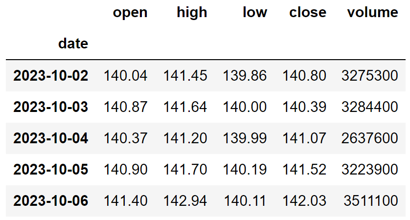
ibm = get_historical_data('IBM', '2020-01-01')
ibm.tail()In the above code, we are using the get_eod_historical_stock_market_data function provided by the eodhd package to extract the split-adjusted historical stock data of IBM. The function consists of the following parameters:
- the
tickerparameter where the symbol of the stock we are interested in extracting the data should be mentioned - the
periodrefers to the time interval between each data point (one-day interval in our case). - the
from_dateandto_dateparameters which indicate the starting and ending date of the data respectively. The format of the input should be “YYYY-MM-DD” - the
orderparameter which is an optional parameter that can be used to order the dataframe either in ascending (a) or descending (d). It is ordered based on the dates.
After extracting the historical data, we are performing some data-wrangling processes to clean and format the data. The final dataframe looks like this:
Step-4: RSI Calculation
In this step, we are going to calculate the values of RSI with 14 as the lookback period using the RSI formula we discussed before.
Python Implementation:
def get_rsi(close, lookback):
ret = close.diff()
up = []
down = []
for i in range(len(ret)):
if ret[i] < 0:
up.append(0)
down.append(ret[i])
else:
up.append(ret[i])
down.append(0)
up_series = pd.Series(up)
down_series = pd.Series(down).abs()
up_ewm = up_series.ewm(com = lookback - 1, adjust = False).mean()
down_ewm = down_series.ewm(com = lookback - 1, adjust = False).mean()
rs = up_ewm/down_ewm
rsi = 100 - (100 / (1 + rs))
rsi_df = pd.DataFrame(rsi).rename(columns = {0:'rsi'}).set_index(close.index)
rsi_df = rsi_df.dropna()
return rsi_df[3:]
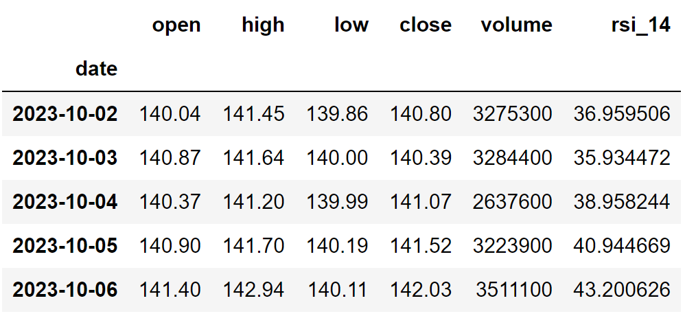
ibm['rsi_14'] = get_rsi(ibm['close'], 14)
ibm = ibm.dropna()
ibm.tail()Output:
Code Explanation: Firstly, we are defining a function named ‘get_rsi’ that takes the closing price of a stock (‘close’) and the lookback period (‘lookback’) as parameters. Inside the function, we are first calculating the returns of the stock using the ‘diff’ function provided by the Pandas package and stored it into the ‘ret’ variable. This function basically subtracts the current value from the previous value. Next, we are passing a for-loop on the ‘ret’ variable to distinguish gains from losses and append those values to the concerning variable (‘up’ or ‘down’).
Then, we are calculating the Exponential Moving Averages for both the ‘up’ and ‘down’ using the ‘ewm’ function provided by the Pandas package and stored them into the ‘up_ewm’ and ‘down_ewm’ variable respectively. Using these calculated EMAs, we are determining the Relative Strength by following the formula we discussed before and stored it into the ‘rs’ variable.
By making use of the calculated Relative Strength values, we are calculating the RSI values by following its formula. After doing some data processing and manipulations, we are returning the calculated Relative Strength Index values in the form of a Pandas dataframe. Finally, we are calling the created function to store the RSI values of IBM with 14 as the lookback period.
Step-4: RSI Plot
In this step, we are going to plot the calculated Relative Strength Index values of IBM to make more sense out of it. The main aim of this part is not on the coding section but instead to observe the plot to gain a solid understanding of RSI.
Python Implementation:
ax1 = plt.subplot2grid((10,1), (0,0), rowspan = 4, colspan = 1)
ax2 = plt.subplot2grid((10,1), (5,0), rowspan = 4, colspan = 1)
ax1.plot(ibm['close'], linewidth = 2.5)
ax1.set_title('IBM CLOSE PRICE')
ax2.plot(ibm['rsi_14'], color = 'orange', linewidth = 2.5)
ax2.axhline(30, linestyle = '--', linewidth = 1.5, color = 'grey')
ax2.axhline(70, linestyle = '--', linewidth = 1.5, color = 'grey')
ax2.set_title('IBM RELATIVE STRENGTH INDEX')
plt.show()
Output:
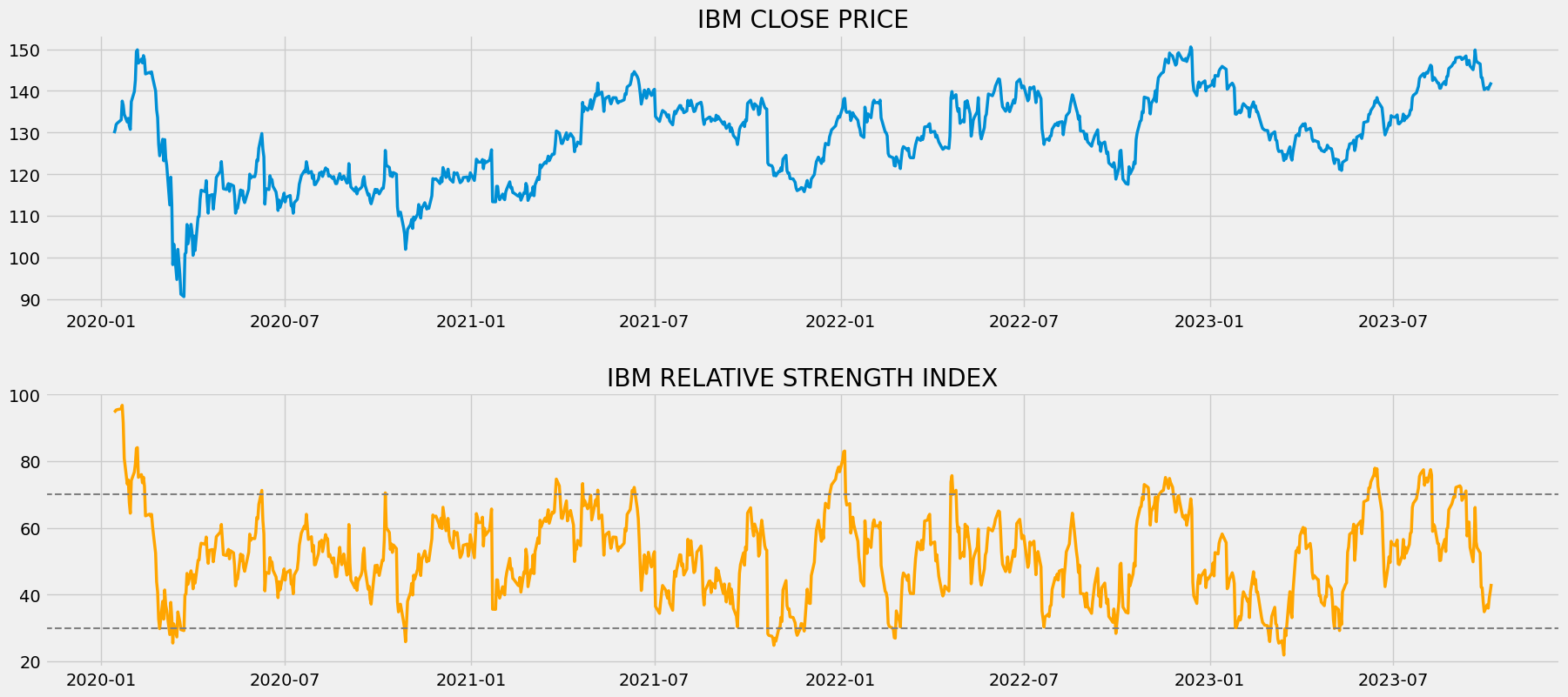
The above chart is separated into two panels: The above panel with the closing price of IBM and the lower panel with the calculated RSI 14 values of IBM. While analyzing the panel plotted with the RSI values, it can be seen that the trend and movement of the calculated values follow the same as the closing price of IBM. So, we can consider that RSI is a directional indicator. Some indicators are non-directional meaning that their movement will be inversely proportional to the actual stock movement and this can sometimes confuse traders and hard to understand too.
While observing the RSI chart, we could see that the plot of RSI reveals trend reversals even before the market does. Simply speaking, the RSI shows a downtrend or an uptrend right before the actual market does. This shows that RSI is a leading indicator. A leading indicator is an indicator that takes into account the current value of a data series to predict future movements. RSI being a leading indicator helps in warning the traders about potential trend reversions before in time. The opposite of leading indicators is called lagging indicators. Lagging indicators are indicators that represent the current value by taking into account the historical values of a data series.
Step-5: Creating the trading strategy
In this step, we are going to implement the discussed Relative Strength Index trading strategy in python.
Python Implementation:
def implement_rsi_strategy(prices, rsi):
    buy_price = []
    sell_price = []
    rsi_signal = []
    signal = 0

    for i in range(len(rsi)):
        if rsi[i-1] > 30 and rsi[i] < 30:
            if signal != 1:
                buy_price.append(prices[i])
                sell_price.append(np.nan)
                signal = 1
                rsi_signal.append(signal)
            else:
                buy_price.append(np.nan)
                sell_price.append(np.nan)
                rsi_signal.append(0)
        elif rsi[i-1] < 70 and rsi[i] > 70:
            if signal != -1:
                buy_price.append(np.nan)
                sell_price.append(prices[i])
                signal = -1
                rsi_signal.append(signal)
            else:
                buy_price.append(np.nan)
                sell_price.append(np.nan)
                rsi_signal.append(0)
        else:
            buy_price.append(np.nan)
            sell_price.append(np.nan)
            rsi_signal.append(0)

    return buy_price, sell_price, rsi_signal

buy_price, sell_price, rsi_signal = implement_rsi_strategy(ibm['close'], ibm['rsi_14'])
Code Explanation: First, we are defining a function named ‘implement_rsi_strategy’ which takes the stock prices (‘prices’), and the RSI values (‘rsi’) as parameters.
Inside the function, we are creating three empty lists (buy_price, sell_price, and rsi_signal) in which the values will be appended while creating the trading strategy.
After that, we are implementing the trading strategy through a for-loop. Inside the for-loop, we are passing certain conditions, and if the conditions are satisfied, the respective values will be appended to the empty lists. If the condition to buy the stock gets satisfied, the buying price will be appended to the ‘buy_price’ list, and the signal value will be appended as 1 representing to buy the stock. Similarly, if the condition to sell the stock gets satisfied, the selling price will be appended to the ‘sell_price’ list, and the signal value will be appended as -1 representing to sell the stock.
Finally, we are returning the lists appended with values. Then, we are calling the created function and stored the values into their respective variables. The list doesn’t make any sense unless we plot the values. So, let’s plot the values of the created trading lists.
Step-6: Plotting the trading signals
In this step, we are going to plot the created trading lists to make sense out of them.
Python Implementation:
ax1 = plt.subplot2grid((10,1), (0,0), rowspan = 4, colspan = 1)
ax2 = plt.subplot2grid((10,1), (5,0), rowspan = 4, colspan = 1)
ax1.plot(ibm['close'], linewidth = 2.5, color = 'skyblue', label = 'ibm')
ax1.plot(ibm.index, buy_price, marker = '^', markersize = 10, color = 'green', label = 'BUY SIGNAL')
ax1.plot(ibm.index, sell_price, marker = 'v', markersize = 10, color = 'r', label = 'SELL SIGNAL')
ax1.set_title('IBM RSI TRADE SIGNALS')
ax2.plot(ibm['rsi_14'], color = 'orange', linewidth = 2.5)
ax2.axhline(30, linestyle = '--', linewidth = 1.5, color = 'grey')
ax2.axhline(70, linestyle = '--', linewidth = 1.5, color = 'grey')
plt.show()
Output:
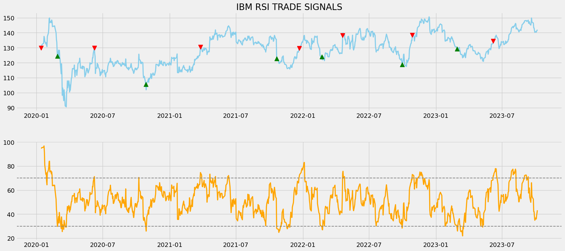
Code Explanation: We are plotting the Relative Strength Index values along with the buy and sell signals generated by the trading strategy. We can observe that whenever the RSI line crosses from above to below the lower band or the oversold level, a green-colored buy signal is plotted in the chart. Similarly, the RSI line crosses from below to above the upper band or the overbought level, a red-colored sell signal is plotted in the chart.
Step-7: Creating our Position
In this step, we are going to create a list that indicates 1 if we hold the stock or 0 if we don’t own or hold the stock.
Python Implementation:
position = []
for i in range(len(rsi_signal)):
    if rsi_signal[i] > 1:
        position.append(0)
    else:
        position.append(1)

for i in range(len(ibm['close'])):
    if rsi_signal[i] == 1:
        position[i] = 1
    elif rsi_signal[i] == -1:
        position[i] = 0
    else:
        position[i] = position[i-1]

rsi = ibm['rsi_14']
close_price = ibm['close']
rsi_signal = pd.DataFrame(rsi_signal).rename(columns = {0:'rsi_signal'}).set_index(ibm.index)
position = pd.DataFrame(position).rename(columns = {0:'rsi_position'}).set_index(ibm.index)

frames = [close_price, rsi, rsi_signal, position]
strategy = pd.concat(frames, join = 'inner', axis = 1)

strategy
Output:
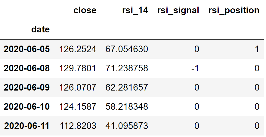
Code Explanation: First, we are creating an empty list named ‘position’. We are passing two for-loops, one is to generate values for the ‘position’ list to just match the length of the ‘signal’ list. The other for-loop is the one we are using to generate actual position values. Inside the second for-loop, we are iterating over the values of the ‘signal’ list, and the values of the ‘position’ list get appended concerning which condition gets satisfied. The value of the position remains 1 if we hold the stock or remains 0 if we sold or don’t own the stock. Finally, we are doing some data manipulations to combine all the created lists into one dataframe.
From the output being shown, we can see that in the first row our position in the stock has remained 1 (since there isn’t any change in the RSI signal) but our position suddenly turned to 0 as we sold the stock when the Relative Strength Index trading signal represents a sell signal (-1). Our position will remain 0 until some changes in the trading signal occur. Now it’s time to do implement some backtesting process!
Step-8: Backtesting
Before moving on, it is essential to know what backtesting is. Backtesting is the process of seeing how well our trading strategy has performed on the given stock data. In our case, we are going to implement a backtesting process for our Relative Strength Index trading strategy over the IBM stock data.
Python Implementation:
ibm_ret = pd.DataFrame(np.diff(ibm['close'])).rename(columns = {0:'returns'})
rsi_strategy_ret = []

for i in range(len(ibm_ret)):
    returns = ibm_ret['returns'][i]*strategy['rsi_position'][i]
    rsi_strategy_ret.append(returns)

rsi_strategy_ret_df = pd.DataFrame(rsi_strategy_ret).rename(columns = {0:'rsi_returns'})
investment_value = 100000
rsi_investment_ret = []

for i in range(len(rsi_strategy_ret_df['rsi_returns'])):
    number_of_stocks = floor(investment_value/ibm['close'][i])
    returns = number_of_stocks*rsi_strategy_ret_df['rsi_returns'][i]
    rsi_investment_ret.append(returns)

rsi_investment_ret_df = pd.DataFrame(rsi_investment_ret).rename(columns = {0:'investment_returns'})
total_investment_ret = round(sum(rsi_investment_ret_df['investment_returns']), 2)
profit_percentage = floor((total_investment_ret/investment_value)*100)
print(cl('Profit gained from the RSI strategy by investing $100k in IBM : {}'.format(total_investment_ret), attrs = ['bold']))
print(cl('Profit percentage of the RSI strategy : {}%'.format(profit_percentage), attrs = ['bold']))
Output:
Profit gained from the RSI strategy by investing $100k in IBM : 69377.53
Profit percentage of the RSI strategy : 69%
Code Explanation: First, we are calculating the returns of the IBM stock using the ‘diff’ function provided by the NumPy package and we have stored it as a dataframe into the ‘ibm_ret’ variable. Next, we are passing a for-loop to iterate over the values of the ‘ibm_ret’ variable to calculate the returns we gained from our Relative Strength Index trading strategy, and these returns values are appended to the ‘rsi_strategy_ret’ list. Next, we are converting the ‘rsi_strategy_ret’ list into a dataframe and stored it into the ‘rsi_strategy_ret_df’ variable.
Next comes the backtesting process. We are going to backtest our strategy by investing a hundred thousand USD into our trading strategy. So first, we are storing the amount of investment into the ‘investment_value’ variable. After that, we are calculating the number of IBM stocks we can buy using the investment amount. You can notice that I’ve used the ‘floor’ function provided by the Math package because, while dividing the investment amount by the closing price of IBM stock, it spits out an output with decimal numbers. The number of stocks should be an integer but not a decimal number. Using the ‘floor’ function, we can cut out the decimals. Remember that the ‘floor’ function is way more complex than the ‘round’ function. Then, we are passing a for-loop to find the investment returns followed by some data manipulations tasks.
Finally, we are printing the total return we got by investing a hundred thousand into our trading strategy and it is revealed that we have made an approximate profit of sixty-nine thousand USD in three years. That’s great!
Final Thoughts!
After a long way of crushing both theories and practical implementations, we have successfully learned what RSI is and how a simple RSI-based trading strategy can be implemented and backtested in python. Even though RSI is one of the most popular trading indicators, it is prone to reveal false signals. Following the false signals and making trades based on those would result in even depleting the capital. Fortunately, there are two ways to keep yourself away from the false signals:
- Additional Indicator: Some stocks might fluctuate a lot and would touch the overbought and oversold levels more frequently. In this case, you should not blindly follow the RSI levels to make your trades but should consider another technical indicator for verifying the signal whether it’s an authentic one or not.
- Strategy Improvisation: The strategy we applied in this article is one of the most basic strategies but there is a lot that can be done with the help of RSI. So, it is highly recommended to have a look at some other trading strategies that are based on the Relative Strength Index before directly diving into the real-world market.
In this article, we didn’t cover either step as the main aim of this article is to just educate people on understanding one of the most important trading indicators, but not to earn profits. There is one more point to remember while using RSI. The Relative Strength Index tends to perform poorly in ranging markets. Ranging markets are markets that show low or no momentum. So, it is highly recommended to stay away from ranging markets while using the Relative Strength Index.
With that being said, you have reached the end of the article. Hope you learned something new and useful.