While I backtested a trading strategy with one of the most popular momentum oscillators, the Moving Average Convergence/Divergence (MACD), the results were amazing. Today, I found a clone of the MACD indicator whose performance is even more efficient. It’s the indicator known as Know Sure Thing, abbreviated as the KST indicator.

In this article, we will first build some basic intuitions on what the KST indicator is all about, and methods to calculate the indicator. After that, we will proceed to the programming part where we use Python to build the indicator from scratch, construct a simple trading strategy based on the indicator, backtest the strategy on Tesla stock and compare its performance with that of SPY ETF (an ETF whose purpose is to track the movements of the S&P 500 market index). With that said, let’s dive into the article!

Quick jump:

1 Rate Of Change (ROC)
2 Know Sure Thing (KST)
3 Implementation in Python
4 Final Thoughts!

Rate Of Change (ROC)

Before moving on to exploring the KST indicator, it is essential to know what the Rate Of Change indicator has got to offer since the Know Sure Thing indicator is based on ROC. The Rate Of Change indicator is a momentum indicator that is used by traders as an instrument to determine the percentage change in price from the current closing price and the price of a specified number of periods ago. Unlike other momentum indicators like the RSI and CCI, the Rate Of Change indicator is an unbounded oscillator whose values do not bound between certain limits.

To calculate the readings of ROC, we have to first determine the ’n’ value which is how many periods ago the current closing price is compared to. The determination of ’n’ varies from one trader to another but the traditional setting is 9 (widely used for short-term trading). With 9 as the ’n’ value, the readings of the ROC indicator are calculated as follows:

First, the closing price of 9 periods ago is subtracted from the current closing price. This difference is then divided by the closing price of 9 periods ago and multiplied by 100. The calculation can be mathematically represented as follows:

ROC 9 = [ ( C.CLOSE - PREV9.CLOSE ) / PREV9.CLOSE ] * 100

where,
C.CLOSE = Current Closing Price
PREV9.CLOSE = Closing Price of 9 Periods ago

Usually, the ROC is plotted below the plot of a stock’s closing price against a zero line. If the readings of the ROC indicator are observed to be above the zero line, then the market is considered to reveal a sturdy upward momentum, and similarly, if the values are below the zero line, the market is considered to reveal a strong downward momentum. This is one way of using the ROC indicator and other usages include generating potential buy and sell signals, identifying the market state (overbought or oversold), and detecting divergences.

That’s what the ROC and its calculation are all about. Now we are ready to jump on to exploring the main idea of this article, the Know Sure Thing indicator.

Know Sure Thing (KST)

The Know Sure Thing indicator is an unbounded momentum oscillator that is widely used by traders to understand the readings of the ROC indicator feasibly. The KST indicator is based on four different timeframes of smoothed ROC and combines the collective data into one oscillator. The Know Sure Thing indicator is composed of two components:

KST line: The first component is the KST line itself. To calculate the readings of the KST line, we have to first determine four ROCs with 10, 15, 20, 30 as the ’n’ values respectively. Then each ROC is smoothed using a Simple Moving Average with 10, 10, 10, 15 as the lookback period respectively. This smoothed ROC is known as ROCSMA. After attaining the ROCSMA for four different timeframes, we have to multiply the first ROCSMA with one, the second ROCSMA with two, the third ROCSMA with three, and the fourth with four. Finally, these four products are added to each other. The calculation of the KST line can be mathematically represented as follows:

KL = (ROCSMA1 * 1) + (ROCSMA2 * 2) + (ROCSMA3 * 3) + (ROCSMA4 * 4)

where,
KL = KST Line
ROCSMA1 = ROC 10 smoothed with SMA 10
ROCSMA2 = ROC 15 smoothed with SMA 10
ROCSMA3 = ROC 20 smoothed with SMA 10
ROCSMA4 = ROC 30 smoothed with SMA 15

Signal line: Now, the second component of the Know Sure Thing indicator is the Signal line component. This component is the smoothed version of the KST line. To smooth the values of the KST line, the Simple Moving Average with 9 as the lookback period is widely used. The calculation of the Signal line looks something as follows:

SIGNAL LINE = SMA9 ( KST LINE )

There are many types of strategies that are built with the KST indicator like the divergence trading strategy, zero line crossover, and so on. Some suggest that it can also be used as an instrument to identify overbought and oversold levels but I personally think that it won’t be as efficient as other indicators like RSI since the KST indicator is an unbounded oscillator. In today’s article, we are going to discuss and implement a basic strategy called the crossover strategy.

The crossover strategy reveals a buy signal whenever the KST line crosses from below to above the Signal line. A sell signal is revealed whenever the KST line crosses from above the below the Signal line. The strategy can be represented as follows:

IF P.KST LINE < P.SIGNAL LINE AND C.KST LINE > C.SIGNAL LINE => BUY
IF P.KST LINE > P.SIGNAL LINE AND C.KST LINE < C.SIGNAL LINE => SELL

This concludes our theory part on the Know Sure Thing indicator. Now, let’s proceed to the programming part where we are going to use python to build the indicator from scratch, construct the crossover trading strategy, backtest the strategy on Tesla stock, compare the crossover strategy returns with those of the SPY ETF. Without further ado, let’s jump into the programming part and do some coding! Before moving on, a note on disclaimer: This article’s sole purpose is to educate people and must be considered as an information piece but not as investment advice.

Implementation in Python

The coding part is classified into various steps as follows:

1. Importing Packages
2. API Key Activation
3. Extracting Historical Stock Data
4. ROC Calculation
5. Know Sure Thing Calculation
6. Know Sure Thing indicator Plot
7. Creating the Trading Strategy
8. Plotting the Trading Lists
9. Creating our Position
10. Backtesting
11. SPY ETF Comparison

We will be following the order mentioned in the above list and buckle up your seat belts to follow every upcoming coding part.

Step-1: Importing Packages

Importing the required packages into the Python environment is a non-skippable step. The primary packages are going to be eodhd for extracting historical stock data, Pandas for data formatting and manipulations, NumPy to work with arrays and for complex functions, and Matplotlib for plotting purposes. The secondary packages are going to be Math for mathematical functions and Termcolor for font customization (optional).

Python Implementation:

# IMPORTING PACKAGES

from eodhd import APIClient
import numpy as np
import matplotlib.pyplot as plt
import pandas as pd
from termcolor import colored as cl
from math import floor

plt.rcParams['figure.figsize'] = (20,10)
plt.style.use('fivethirtyeight')

With the required packages imported into Python, we can proceed to fetch historical data for Tesla using EODHD’s eodhd Python library. Also, if you haven’t installed any of the imported packages, make sure to do so using the pip command in your terminal.

Step-2: API Key Activation

It is essential to register the EODHD API key with the package in order to use its functions. If you don’t have an EODHD API key, firstly, head over to their website, then, finish the registration process to create an EODHD account, and finally, navigate to the ‘Settings’ page where you could find your secret EODHD API key. It is important to ensure that this secret API key is not revealed to anyone. You can activate the API key by following this code:

api_key = '<YOUR API KEY>'
client = APIClient(api_key)

The code is pretty simple. In the first line, we are storing the secret EODHD API key into the api_key and then in the second line, we are using the APIClient class provided by the eodhd package to activate the API key and stored the response in the client variable.

Note that you need to replace <YOUR API KEY> with your secret EODHD API key. Apart from directly storing the API key with text, there are other ways for better security such as utilizing environmental variables, and so on.

Step-3: Extracting Historical Stock Data

Before heading into the extraction part, it is first essential to have some background about historical or end-of-day data. In a nutshell, historical data consists of information accumulated over a period of time. It helps in identifying patterns and trends in the data. It also assists in studying market behavior. Now, you can easily extract the historical data of any tradeable assets using the eod package by following this code:

# EXTRACTING HISTORICAL DATA

def extract_historical_data(ticker, start_date):
    json_resp = client.get_eod_historical_stock_market_data(symbol = ticker, period = 'd', from_date = start_date, order = 'a')
    df = pd.DataFrame(json_resp)
    df = df.set_index('date')
    df.index = pd.to_datetime(df.index)
    return df

tsla = get_historical_data('TSLA', '2019-01-01')
tsla.tail()

In the above code, we are using the get_eod_historical_stock_market_data function provided by the eodhd package to extract the split-adjusted historical stock data of Tesla. The function consists of the following parameters:

the ticker parameter where the symbol of the stock we are interested in extracting the data should be mentioned
the period refers to the time interval between each data point (one-day interval in our case).
the from_date and to_date parameters which indicate the starting and ending date of the data respectively. The format of the input should be “YYYY-MM-DD”
the order parameter which is an optional parameter that can be used to order the dataframe either in ascending (a) or descending (d). It is ordered based on the dates.

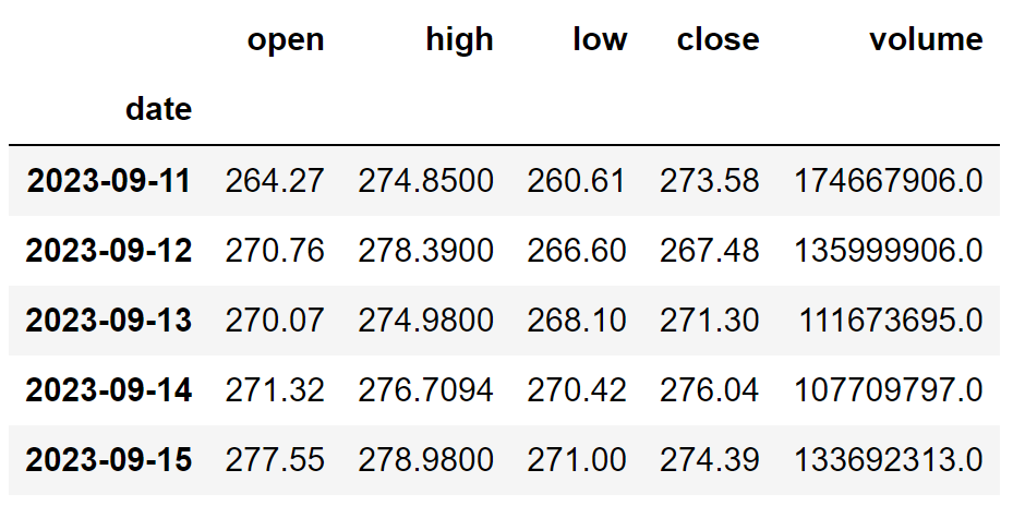
After extracting the historical data, we are performing some data-wrangling processes to clean and format the data. The final dataframe looks like this:

Step-4: ROC Calculation

In this step, we are going to define a function to calculate the values of the Rate Of Change Indicator for a given series.

Python Implementation:

# ROC CALCULATION

def get_roc(close, n):
    difference = close.diff(n)
    nprev_values = close.shift(n)
    roc = (difference / nprev_values) * 100
    return roc

Code Explanation: We are first defining a function named ‘get_roc’ that takes the stock’s closing price (‘close’) and the ’n’ value (‘n’) as parameters. Inside the function, we are first taking the difference between the current closing price and the closing price for a specified number of periods ago using the ‘diff’ function provided by the Pandas package. With the help of the ‘shift’ function, we are taking into account the closing price for a specified number of periods ago and stored it into the ‘nprev_values’ variable. Then, we are substituting the determined values into the ROC indicator formula we discussed before to calculate the values and finally returned the data.

Step-5: Know Sure Thing Calculation

In this step, we are going to calculate the components of the Know Sure Thing indicator by following the methods and formulas we discussed before.

Python Implementation:

# KST CALCULATION

def get_kst(close, sma1, sma2, sma3, sma4, roc1, roc2, roc3, roc4, signal):
    rcma1 = get_roc(close, roc1).rolling(sma1).mean()
    rcma2 = get_roc(close, roc2).rolling(sma2).mean()
    rcma3 = get_roc(close, roc3).rolling(sma3).mean()
    rcma4 = get_roc(close, roc4).rolling(sma4).mean()
    kst = (rcma1 * 1) + (rcma2 * 2) + (rcma3 * 3) + (rcma4 * 4)
    signal = kst.rolling(signal).mean()
    return kst, signal

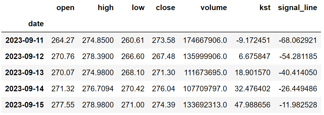
tsla['kst'], tsla['signal_line'] = get_kst(tsla['close'], 10, 10, 10, 15, 10, 15, 20, 30, 9)
tsla = tsla[tsla.index >= '2020-01-01']
tsla.tail()

Output:

Code Explanation: Firstly, we are defining a function named ‘get_kst’ that takes the closing price of the stock (‘close’), four lookback periods for smoothing the ROC values (‘sma1’, ‘sma2’, ‘sma3’, ‘sma4’), four ’n’ values of ROC (‘roc1’, ‘roc2’, ‘roc3’, ‘roc4’), and the lookback period for the signal line (‘signal’) as parameters.

Inside the function, we are first calculating the four ROCSMA values using the ‘rolling’ function provided by the Pandas package and the ‘get_roc’ function we created previously. Then, we are substituting the calculated ROCSMAs into the formula we discussed before to determine the readings of the KST line. Then, we smoothed the KST line values with the ‘rolling’ function to get the values of the Signal line and stored them in the ‘signal’ variable.

Finally, we are returning both the calculated components of the KST indicator and calling the created function to store Tesla’s KST line and the Signal line readings.

Step-6: Know Sure Thing indicator Plot

In this step, we are going to plot the calculated components of the KST indicator values of Tesla to make more sense of them. The main aim of this part is not on the coding section but instead to observe the plot to gain a solid understanding of the Know Sure Thing technical indicator.

Python Implementation:

# KST INDICATOR PLOT

ax1 = plt.subplot2grid((11,1), (0,0), rowspan = 5, colspan = 1)
ax2 = plt.subplot2grid((11,1), (6,0), rowspan = 5, colspan = 1)
ax1.plot(tsla['close'], linewidth = 2.5)
ax1.set_title('TSLA CLOSING PRICES')
ax2.plot(tsla['kst'], linewidth = 2, label = 'KST', color = 'orange')
ax2.plot(tsla['signal_line'], linewidth = 2, label = 'SIGNAL', color = 'mediumorchid')
ax2.legend()
ax2.set_title('TSLA KST')
plt.show()

Output:

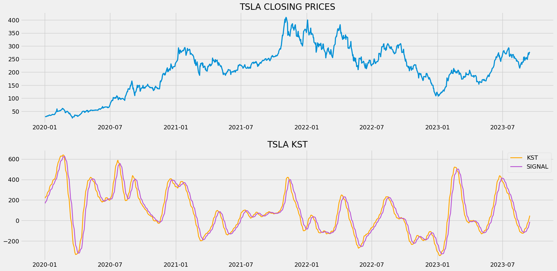
The above chart is divided into two panels: The upper panel with the closing price of Tesla, and the lower panel with the components of the Know Sure Thing Indicator. It can be noticed that the readings of both components are indefinite and not bounded between certain limits because the Know Sure Thing indicator is an unbounded oscillator. This is the reason for the absence of the overbought and oversold levels in the chart that is widely plotted in other momentum oscillators. However, some propose that this indicator can be used to determine overbought and oversold levels but differ from one stock to another. This means, unlike other momentum oscillators which have default overbought and oversold levels, it is necessary to analyze the movement and readings of KST’s components to determine the overbought and oversold levels. In our case, it would be optimal to spot the overbought level at 100 and the oversold level at -100.

One special characteristic feature of the KST indicator is that apart from determining the overbought and oversold levels or spotting divergence, it can be used as a tool to detect ranging markets (markets that show no trend or momentum but move back and forth between specific high and low price ranges). Whenever both the components cross back and forth to each other, then the market is considered to be ranging. As Tesla’s stock shows huge price movements, this phenomenon can be observed only a very few times (actually two: one around June and July in the previous year, the other at the start of 2021).

Step-7: Creating the trading strategy

In this step, we are going to implement the discussed Know Sure Thing crossover trading strategy in Python.

Python Implementation:

# KST CROSSOVER TRADING STRATEGY

def implement_kst_strategy(prices, kst_line, signal_line):
    buy_price = []
    sell_price = []
    kst_signal = []
    signal = 0
    
    for i in range(len(kst_line)):
        
        if kst_line[i-1] < signal_line[i-1] and kst_line[i] > signal_line[i]:
            if signal != 1:
                buy_price.append(prices[i])
                sell_price.append(np.nan)
                signal = 1
                kst_signal.append(signal)
            else:
                buy_price.append(np.nan)
                sell_price.append(np.nan)
                kst_signal.append(0)
                
        elif kst_line[i-1] > signal_line[i-1] and kst_line[i] < signal_line[i]:
            if signal != -1:
                buy_price.append(np.nan)
                sell_price.append(prices[i])
                signal = -1
                kst_signal.append(signal)
            else:
                buy_price.append(np.nan)
                sell_price.append(np.nan)
                kst_signal.append(0)
                
        else:
            buy_price.append(np.nan)
            sell_price.append(np.nan)
            kst_signal.append(0)
            
    return buy_price, sell_price, kst_signal

buy_price, sell_price, kst_signal = implement_kst_strategy(tsla['close'], tsla['kst'], tsla['signal_line'])

Code Explanation: First, we are defining a function named ‘implement_kst_strategy’ which takes the stock prices (‘prices’), the readings of the KST line (‘kst_line’), and the readings of the Signal line (‘signal_line’) as parameters.

Inside the function, we are creating three empty lists (buy_price, sell_price, and kst_signal) in which the values will be appended while creating the trading strategy.

After that, we are implementing the trading strategy through a for-loop. Inside the for-loop, we are passing certain conditions, and if the conditions are satisfied, the respective values will be appended to the empty lists. If the condition to buy the stock is satisfied, the buying price will be appended to the ‘buy_price’ list, and the signal value will be appended as 1 representing buying the stock. Similarly, if the condition to sell the stock is satisfied, the selling price will be appended to the ‘sell_price’ list, and the signal value will be appended as -1 representing to sell the stock.

Finally, we are returning the lists appended with values. Then, we call the created function and store the values in their respective variables. The list doesn’t make any sense unless we plot the values. So, let’s plot the values of the created trading lists.

Step-8: Plotting the trading signals

In this step, we are going to plot the created trading lists to make sense of them.

Python Implementation:

# TRADING SIGNALS PLOT

ax1 = plt.subplot2grid((11,1), (0,0), rowspan = 5, colspan = 1)
ax2 = plt.subplot2grid((11,1), (6,0), rowspan = 5, colspan = 1)
ax1.plot(tsla['close'], linewidth = 2, label = 'TSLA')
ax1.plot(tsla.index, buy_price, marker = '^', markersize = 12, linewidth = 0, color = 'green', label = 'BUY SIGNAL')
ax1.plot(tsla.index, sell_price, marker = 'v', markersize = 12, linewidth = 0, color = 'r', label = 'SELL SIGNAL')
ax1.legend()
ax1.set_title('TSLA KST TRADING SIGNALS')
ax2.plot(tsla['kst'], linewidth = 2, label = 'KST', color = 'orange')
ax2.plot(tsla['signal_line'], linewidth = 2, label = 'SIGNAL', color = 'mediumorchid')
ax2.legend()
ax2.set_title('TSLA KST')
plt.show()

Output:

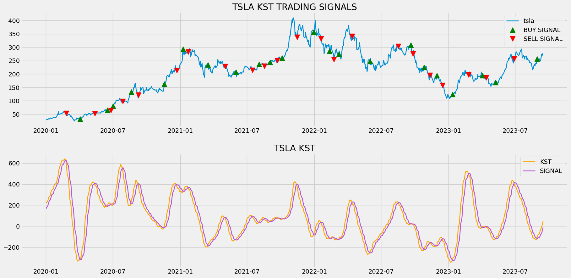
Code Explanation: We are plotting the readings of the KST indicator’s components along with the buy and sell signals generated by the crossover trading strategy. We can observe that whenever the KST line crosses from below to above the Signal line, a green-colored buy signal is plotted in the chart. Similarly, whenever the KST line crosses from above to below the Signal line, a red-colored sell signal is plotted in the chart.

Step-9: Creating our Position

In this step, we are going to create a list that indicates 1 if we hold the stock or 0 if we don’t own or hold the stock.

Python Implementation:

# STOCK POSITION

position = []
for i in range(len(kst_signal)):
    if kst_signal[i] > 1:
        position.append(0)
    else:
        position.append(1)
        
for i in range(len(tsla['close'])):
    if kst_signal[i] == 1:
        position[i] = 1
    elif kst_signal[i] == -1:
        position[i] = 0
    else:
        position[i] = position[i-1]
        
close_price = tsla['close']
kst = tsla['kst']
signal_line = tsla['signal_line']
kst_signal = pd.DataFrame(kst_signal).rename(columns = {0:'kst_signal'}).set_index(tsla.index)
position = pd.DataFrame(position).rename(columns = {0:'kst_position'}).set_index(tsla.index)

frames = [close_price, kst, signal_line, kst_signal, position]
strategy = pd.concat(frames, join = 'inner', axis = 1)

strategy

Output:

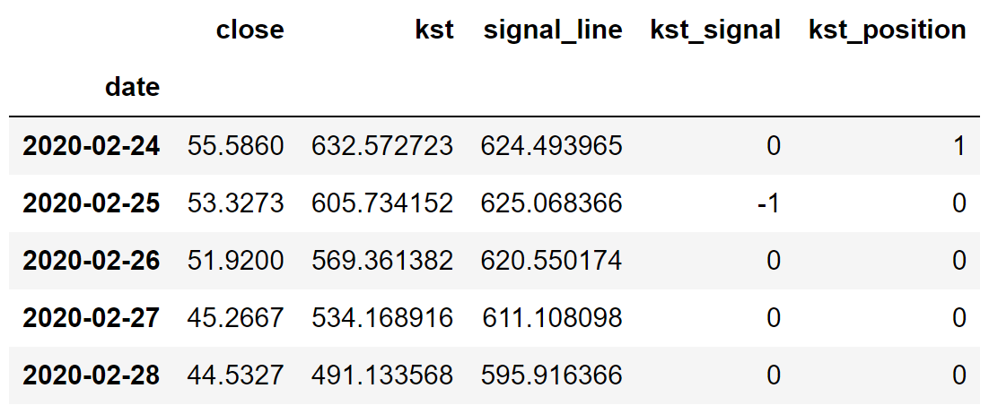
Code Explanation: First, we are creating an empty list named ‘position’. We are passing two for-loops, one is to generate values for the ‘position’ list to just match the length of the ‘signal’ list. The other for-loop is the one we are using to generate actual position values. Inside the second for-loop, we are iterating over the values of the ‘signal’ list, and the values of the ‘position’ list get appended concerning which condition gets satisfied. The value of the position remains 1 if we hold the stock or remains 0 if we sold or don’t own the stock. Finally, we are doing some data manipulations to combine all the created lists into one dataframe.

From the output being shown, we can see that in the first row our position in the stock has remained 1 (since there isn’t any change in the KST signal) but our position suddenly turned to -1 as we sold the stock when the KST trading signal represents a sell signal (-1). Our position will remain 0 until some changes in the trading signal occur. Now it’s time to do implement some backtesting process!

Step-10: Backtesting

Before moving on, it is essential to know what backtesting is. Backtesting is the process of seeing how well our trading strategy has performed on the given stock data. In our case, we are going to implement a backtesting process for our KST indicator crossover trading strategy over the Tesla stock data.

Python Implementation:

# BACKTESTING

tsla_ret = pd.DataFrame(np.diff(tsla['close'])).rename(columns = {0:'returns'})
kst_strategy_ret = []for i in range(len(tsla_ret)):
    returns = tsla_ret['returns'][i]*strategy['kst_position'][i]
    kst_strategy_ret.append(returns)
    
kst_strategy_ret_df = pd.DataFrame(kst_strategy_ret).rename(columns = {0:'kst_returns'})
investment_value = 100000
kst_investment_ret = []

for i in range(len(kst_strategy_ret_df['kst_returns'])):
    number_of_stocks = floor(investment_value/tsla['close'][i])
    returns = number_of_stocks*kst_strategy_ret_df['kst_returns'][i]
    kst_investment_ret.append(returns)

kst_investment_ret_df = pd.DataFrame(kst_investment_ret).rename(columns = {0:'investment_returns'})
total_investment_ret = round(sum(kst_investment_ret_df['investment_returns']), 2)
profit_percentage = floor((total_investment_ret/investment_value)*100)
print(cl('Profit gained from the KST strategy by investing $100k in TSLA : {}'.format(total_investment_ret), attrs = ['bold']))
print(cl('Profit percentage of the KST strategy : {}%'.format(profit_percentage), attrs = ['bold']))

Output:

Profit gained from the KST strategy by investing $100k in TSLA : 281648.14
Profit percentage of the KST strategy : 281%

Code Explanation: First, we are calculating the returns of the Tesla stock using the ‘diff’ function provided by the NumPy package and we have stored it as a dataframe into the ‘tsla_ret’ variable. Next, we are passing a for-loop to iterate over the values of the ‘tsla_ret’ variable to calculate the returns we gained from our Know Sure Thing indicator trading strategy, and these returns values are appended to the ‘kst_strategy_ret’ list. Next, we are converting the ‘kst_strategy_ret’ list into a dataframe and stored it into the ‘kst_strategy_ret_df’ variable.

Next comes the backtesting process. We are going to backtest our strategy by investing a hundred thousand USD into our trading strategy. So first, we are storing the amount of investment into the ‘investment_value’ variable. After that, we are calculating the number of Tesla stocks we can buy using the investment amount. You can notice that I’ve used the ‘floor’ function provided by the Math package because, while dividing the investment amount by the closing price of Tesla stock, it spits out an output with decimal numbers. The number of stocks should be an integer but not a decimal number. Using the ‘floor’ function, we can cut out the decimals. Remember that the ‘floor’ function is way more complex than the ‘round’ function. Then, we pass a for-loop to find the investment returns followed by some data manipulation tasks.

Finally, we are printing the total return we got by investing a hundred thousand into our trading strategy and it is revealed that we have made an approximate profit of two hundred and eighty-one thousand USD in one year. That’s awesome! Now, let’s compare our returns with SPY ETF (an ETF designed to track the S&P 500 stock market index) returns.

Step-11: SPY ETF Comparison

This step is optional but it is highly recommended as we can get an idea of how well our trading strategy performs against a benchmark (SPY ETF). In this step, we are going to extract the data of the SPY ETF using the ‘get_historical_data’ function we created and compare the returns we get from the SPY ETF with our KST crossover trading strategy returns on Tesla.

Python Implementation:

# SPY ETF COMPARISON

def get_benchmark(start_date, investment_value):
    spy = get_historical_data('SPY', start_date)['close']
    benchmark = pd.DataFrame(np.diff(spy)).rename(columns = {0:'benchmark_returns'})
    
    investment_value = investment_value
    benchmark_investment_ret = []
    
    for i in range(len(benchmark['benchmark_returns'])):
        number_of_stocks = floor(investment_value/spy[i])
        returns = number_of_stocks*benchmark['benchmark_returns'][i]
        benchmark_investment_ret.append(returns)

    benchmark_investment_ret_df = pd.DataFrame(benchmark_investment_ret).rename(columns = {0:'investment_returns'})
    return benchmark_investment_ret_df

benchmark = get_benchmark('2020-01-01', 100000)
investment_value = 100000
total_benchmark_investment_ret = round(sum(benchmark['investment_returns']), 2)
benchmark_profit_percentage = floor((total_benchmark_investment_ret/investment_value)*100)
print(cl('Benchmark profit by investing $100k : {}'.format(total_benchmark_investment_ret), attrs = ['bold']))
print(cl('Benchmark Profit percentage : {}%'.format(benchmark_profit_percentage), attrs = ['bold']))
print(cl('KST Strategy profit is {}% higher than the Benchmark Profit'.format(profit_percentage - benchmark_profit_percentage), attrs = ['bold']))

Output:

Benchmark profit by investing $100k : 41144.52
Benchmark Profit percentage : 41%
KST Strategy profit is 240% higher than the Benchmark Profit

Code Explanation: The code used in this step is almost similar to the one used in the previous backtesting step but, instead of investing in Tesla, we are investing in SPY ETF by not implementing any trading strategies. From the output, we can see that our Know Sure Thing crossover trading strategy has outperformed the SPY ETF by 240%. That’s great!

Final Thoughts!

After an overwhelming process of crushing both theory and coding parts, we have successfully learned what the Know Sure Thing indicator is all about, the math behind it, and how to build a simple KST crossover trading strategy in Python.

Even though we made a wonderful profit with our KST strategy and outperformed the SPY ETF, our strategy returns are still lesser than the actual Tesla stock returns. This is because of one major drawback of the KST indicator. That is the KST indicator is prone to revealing a lot of false signals during the periods of ranging markets and this can be observed in our crossover trading signal plot where a lot of unnecessary trading signals are revealed by our trading strategy.

The only way to optimize and resolve this problem is by adding another technical indicator that acts as a gauge to filter non-authentic or false signals given by the trading strategy. In my opinion, the Choppiness Index would work wonderfully with the KST indicator since it is an indicator dedicated to tracking whether a market is ranging or not, also, it is one of the most accurate indicators to do so. So it is highly recommended to run as many backtests as possible with a KST trading strategy that uses another indicator to differentiate the false signals from the authentic ones and doing this will take your results to the next level.

With that being said, you’ve reached the end of the article. If you forgot to follow any of the coding parts, don’t worry. Happy learning!

Rate Of Change (ROC)

Know Sure Thing (KST)

Implementation in Python

Step-1: Importing Packages

Step-2: API Key Activation

Step-3: Extracting Historical Stock Data

Step-4: ROC Calculation

Step-5: Know Sure Thing Calculation

Step-6: Know Sure Thing indicator Plot

Step-7: Creating the trading strategy

Step-8: Plotting the trading signals

Step-9: Creating our Position

Step-10: Backtesting

Step-11: SPY ETF Comparison

Final Thoughts!

Related Articles

Backtesting Technical Analysis Strategies with Excel(SMA, RSI, MACD)

Using Delisted Stocks for Backtesting a 3-EMA Strategy with Python

Practical Guide to Automated Detection Trading Patterns with Python

Benchmark Tracking and Cointegration Analysis with Python

Backtesting a Killer Mean Reversion Trading Strategy with Python

Maximising Profits Trading with Moving Average Crossovers