While having a look at the list of most popular momentum indicators that consists of the Relative Strength Index, and the Stochastic Oscillator, the one we are going to discuss today also joins the list when considering its usage and efficiency in the real world market. It’s an indicator known as Williams %R.

In this article, we are going to explore what Williams %R is all about, the math behind this indicator, and how a trading strategy based on it can be built with the help of Python. As a bonus step, we will compare the returns of our Williams %R strategy returns with the returns of SPY ETF (an ETF specifically designed to track the movement of the S&P 500 Index) to get an idea of how well our strategy performs in the real-world market and can be considered as a step to evaluate the strategy. Considering your curiosity piqued, let’s dive into the article!

Quick jump:

1 Williams %R
2 Implementation in Python
3 Final Thoughts!

Williams %R

Founded by Larry Williams, the Williams %R is a momentum indicator whose values oscillate between 0 to -100. This indicator is most similar to the Stochastic Oscillator, but differs in its calculation. Traders use this indicator to spot potential entry and exit points for trades by constructing two levels of overbought and oversold. Before moving on, a word on overbought and oversold levels: A stock is said to be overbought when the market’s trend seems to be extremely bullish and bound to consolidate. Similarly, a stock reaches an oversold region when the market’s trend seems to be extremely bearish and has the tendency to bounce. The traditional threshold for overbought and oversold levels are 20 and 80 respectively but there aren’t any prohibitions in taking other values too.

In order to calculate the values of Williams %R with the traditional setting of 14 as the lookback period, first, the highest high and the lowest low for each period over a fourteen-day timeframe is determined. Then, the two differences are taken: The closing price from the highest high, and the lowest low from the highest high. Finally, the first difference is divided by the second difference and multiple by -100 to obtain the values of Williams %R. The calculation can be mathematically represented as follows:

W%R 14 = [ H.HIGH - C.PRICE ] / [ L.LOW - C.PRICE ] * ( - 100 )

where,
W%R 14 = 14-day Williams %R of the stock
H.HIGH = 14-day Highest High of the stock
L.LOW = 14-day Lowest Low of the stock
C.PRICE = Closing price of the stock

The underlying idea of this indicator is that the stock will keep reaching new highs when it is a strong uptrend and similarly, the stock will reach new lows when it follows a sturdy downtrend. With that being said, let’s discuss the trading strategy we are going to implement in this article.

About our trading strategy: There are a lot of Williams %R-based trading strategies that can be implemented in the real world market but the one we are going to discuss today is a strategy based on the overbought and oversold levels. The strategy reveals a buy signal whenever the previous reading of the Williams %R is below -20 and the current reading is above -20. Likewise, a sell signal is generated whenever the previous reading of the Williams %R is above -80 and the current reading is below -80. Our trading strategy can be represented as follows:

IF PREV.W%R < [ - 20 ] AND CURRENT.W%R > [ - 20 ] ==> BUY SIGNAL
IF PREV.W%R > [ - 80 ] AND CURRENT.W%R < [ - 80 ] ==> SELL SIGNAL

This concludes our theory part on Williams %R, its calculation, and the trading strategy. Now, let’s build this indicator from scratch in Python, construct the trading strategy we discussed, backtest it on the Netflix data, and compare the returns with those of the SPY ETF. Without further ado, let’s do some coding! Before moving on, a note on disclaimer: This article’s sole purpose is to educate people and must be considered as an information piece but not as investment advice.

Implementation in Python

The coding part is classified into various steps as follows:

1. Importing Packages
2. API Key Activation
2. Extracting Historical Stock Data
3. Williams %R Calculation
4. Williams %R Indicator Plot
5. Creating the Trading Strategy
6. Plotting the Trading Lists
7. Creating our Position
8. Backtesting
9. SPY ETF Comparison

We will be following the order mentioned in the above list and buckle up your seat belts to follow every upcoming coding part.

Step-1: Importing Packages

Importing the required packages into the Python environment is a non-skippable step. The primary packages are going to be eodhd for extracting historical stock data, Pandas for data formatting and manipulations, NumPy to work with arrays and for complex functions, and Matplotlib for plotting purposes. The secondary packages are going to be Math for mathematical functions and Termcolor for font customization (optional).

Python Implementation:

# IMPORTING PACKAGES

import numpy as np
import matplotlib.pyplot as plt
import pandas as pd
from termcolor import colored as cl
from math import floor
from eodhd import APIClient

plt.rcParams['figure.figsize'] = (20,10)
plt.style.use('fivethirtyeight')

With the required packages imported into Python, we can proceed to fetch historical data for Netflix using EODHD’s eodhd Python library. Also, if you haven’t installed any of the imported packages, make sure to do so using the pip command in your terminal.

Step-2: API Key Activation

It is essential to register the EODHD API key with the package in order to use its functions. If you don’t have an EODHD API key, firstly, head over to their website, then, finish the registration process to create an EODHD account, and finally, navigate to the ‘Settings’ page where you could find your secret EODHD API key. It is important to ensure that this secret API key is not revealed to anyone. You can activate the API key by following this code:

api_key = '<YOUR API KEY>'
client = APIClient(api_key)

The code is pretty simple. In the first line, we are storing the secret EODHD API key into the api_key and then in the second line, we are using the APIClient class provided by the eodhd package to activate the API key and stored the response in the client variable.

Note that you need to replace <YOUR API KEY> with your secret EODHD API key. Apart from directly storing the API key with text, there are other ways for better security such as utilizing environmental variables, and so on.

Step-3: Extracting Historical Data

Before heading into the extraction part, it is first essential to have some background about historical or end-of-day data. In a nutshell, historical data consists of information accumulated over a period of time. It helps in identifying patterns and trends in the data. It also assists in studying market behavior. Now, you can easily extract the historical data of any tradeable assets using the eod package by following this code:

# EXTRACTING HISTORICAL DATA

def extract_historical_data(ticker, start_date):
    json_resp = client.get_eod_historical_stock_market_data(symbol = ticker, period = 'd', from_date = start_date, order = 'a')
    df = pd.DataFrame(json_resp)
    df = df.set_index('date')
    df.index = pd.to_datetime(df.index)
    return df

nflx = get_historical_data('NFLX', '2020-01-01')
nflx.tail()

In the above code, we are using the get_eod_historical_stock_market_data function provided by the eod package to extract the split-adjusted historical stock data of Netflix. The function consists of the following parameters:

the ticker parameter where the symbol of the stock we are interested in extracting the data should be mentioned
the period refers to the time interval between each data point (one-day interval in our case).
the from_date and to_date parameters which indicate the starting and ending date of the data respectively. The format of the input should be “YYYY-MM-DD”
the order parameter which is an optional parameter that can be used to order the dataframe either in ascending (a) or descending (d). It is ordered based on the dates.

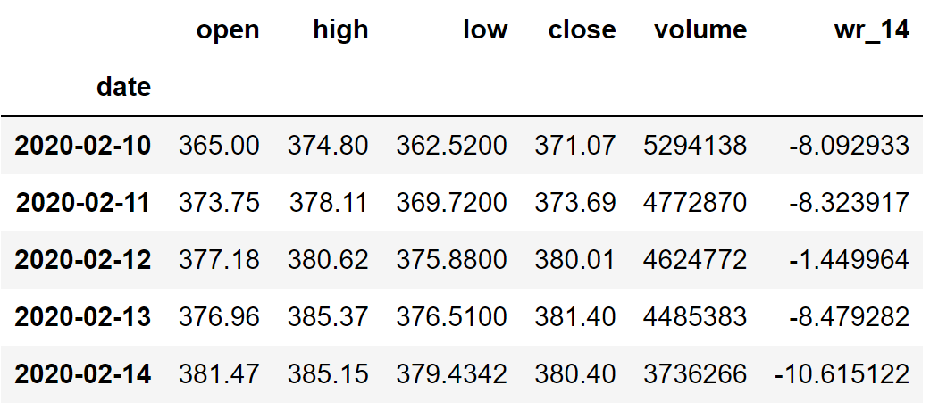
After extracting the historical data, we are performing some data-wrangling processes to clean and format the data. The final dataframe looks like this:

Step-3: Williams %R Calculation

In this step, we are going to calculate the values of Williams %R by following the formula we discussed before.

Python Implementation:

def get_wr(high, low, close, lookback):
    highh = high.rolling(lookback).max() 
    lowl = low.rolling(lookback).min()
    wr = -100 * ((highh - close) / (highh - lowl))
    return wr

nflx['wr_14'] = get_wr(nflx['high'], nflx['low'], nflx['close'], 14)
nflx = nflx.dropna()
nflx.head()

Output:

Code Explanation: We are first defining a function named ‘get_wr’ that takes a stock’s high price data (‘high’), low price data (‘low’), closing price data (‘close’), and the lookback period (‘period’) as parameters. Inside the function, we are first determining the highest high over a specific lookback period timeframe with the help of the ‘rolling’ and ‘max’ functions provided by the Pandas package and stored it into the ‘highh’ variable. What the ‘rolling’ function performs is that it will take into account the n-period timeframe we specify and the ‘max’ function filters the maximum values present in the given dataframe.

Next, we are defining a variable named ‘lowl’ to store the lowest low over a specified lookback period timeframe which we determined using the ‘rolling’ and ‘min’ function (as the name suggests, filters the minimum values in the given dataframe) provided by the Pandas package.

Then, we are substituting the determined highest high and lowest low values into the formula we discussed before to calculate the values of Williams %R and stored it into the ‘wr’ variable. Finally, we are returning and calling the created function to store Netflix’s Williams %R readings with 14 as the lookback period.

Step-4: Williams %R Plot

In this step, we are going to plot the calculated Williams %R values of Netflix to make more sense of them. The main aim of this part is not on the coding section but instead to observe the plot to gain a solid understanding of the Williams %R technical indicator.

Python Implementation:

ax1 = plt.subplot2grid((11,1), (0,0), rowspan = 5, colspan = 1)
ax2 = plt.subplot2grid((11,1), (6,0), rowspan = 5, colspan = 1)
ax1.plot(nflx['close'], linewidth = 2)
ax1.set_title('NFLX CLOSING PRICE')
ax2.plot(nflx['wr_14'], color = 'orange', linewidth = 2)
ax2.axhline(-20, linewidth = 1.5, linestyle = '--', color = 'grey')
ax2.axhline(-80, linewidth = 1.5, linestyle = '--', color = 'grey')
ax2.set_title('NFLX WILLIAMS %R 14')
plt.show()

Output:

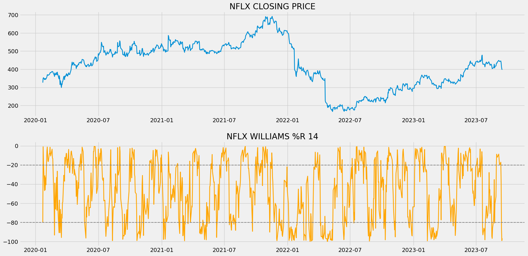
The above chart is divided into two panels: The upper panel with the closing price of Netflix’s stock data and the lower panel with the values of Netflix’s 14-day readings of Williams %R. Now, the chart can be utilized in two ways. The first way is using the chart as a tool to identify overbought and oversold states of the market. You could observe that there are two horizontal grey lines plotted above and below the market which are the overbought and oversold levels plotted at a threshold of -20 and -80 respectively. You can consider that the market is in the state of overbought if the Williams %R has a reading of above the upper line or the overbought line. Similarly, you can assume that the market is in the state of oversold if the Williams %R has a reading of below the lower line or the oversold line.

The second way of using Williams %R is to identify false momentum in the market. During a sturdy uptrend, the readings of Williams %R tend to reach above -20 frequently. If the indicator falls and struggles to reach above -20 before the next fall, indicates that the market’s momentum is not authentic and possible to follow a tremendous downtrend. Likewise, during a healthy downtrend, the readings of Williams %R bound to go below -80 frequently. If the indicator rises and fails to reach -80 before the next rise, reveals that the market is going to follow a positive trend.

Since Williams %R is a directional indicator (an indicator whose movement is directly proportional to that of the actual market), traders also use this indicator to find and confirm strong uptrends or downtrends in a market and trade along with it. Some indicators are not of much use while utilized for identifying or confirming market trends as they might be lagging in nature (an indicator that takes into account the historical data points to determine the current reading) but Williams %R is an effective one because it is a leading indicator (an indicator that takes into account the previous data points to predict the future movements).

Step-5: Creating the trading strategy

In this step, we are going to implement the discussed Williams %R trading strategy in Python.

Python Implementation:

def implement_wr_strategy(prices, wr):    
    buy_price = []
    sell_price = []
    wr_signal = []
    signal = 0

    for i in range(len(wr)):
        if wr[i-1] > -80 and wr[i] < -80:
            if signal != 1:
                buy_price.append(prices[i])
                sell_price.append(np.nan)
                signal = 1
                wr_signal.append(signal)
            else:
                buy_price.append(np.nan)
                sell_price.append(np.nan)
                wr_signal.append(0)
        elif wr[i-1] < -20 and wr[i] > -20:
            if signal != -1:
                buy_price.append(np.nan)
                sell_price.append(prices[i])
                signal = -1
                wr_signal.append(signal)
            else:
                buy_price.append(np.nan)
                sell_price.append(np.nan)
                wr_signal.append(0)
        else:
            buy_price.append(np.nan)
            sell_price.append(np.nan)
            wr_signal.append(0)
            
    return buy_price, sell_price, wr_signal
            
buy_price, sell_price, wr_signal = implement_wr_strategy(nflx['close'], nflx['wr_14'])

Code Explanation: First, we are defining a function named ‘implement_wr_strategy’ which takes the stock prices (‘prices’), and the values of Williams %R indicator (‘wr’) as parameters.

Inside the function, we are creating three empty lists (buy_price, sell_price, and wr_signal) in which the values will be appended while creating the trading strategy.

After that, we are implementing the trading strategy through a for-loop. Inside the for-loop, we are passing certain conditions, and if the conditions are satisfied, the respective values will be appended to the empty lists. If the condition to buy the stock gets satisfied, the buying price will be appended to the ‘buy_price’ list, and the signal value will be appended as 1 representing to buy the stock. Similarly, if the condition to sell the stock gets satisfied, the selling price will be appended to the ‘sell_price’ list, and the signal value will be appended as -1 representing to sell the stock.

Finally, we are returning the lists appended with values. Then, we are calling the created function and stored the values into their respective variables. The list doesn’t make any sense unless we plot the values. So, let’s plot the values of the created trading lists.

Step-6: Plotting the trading signals

In this step, we are going to plot the created trading lists to make sense of them.

Python Implementation:

ax1 = plt.subplot2grid((11,1), (0,0), rowspan = 5, colspan = 1)
ax2 = plt.subplot2grid((11,1), (6,0), rowspan = 5, colspan = 1)
ax1.plot(nflx['close'], linewidth = 2)
ax1.plot(nflx.index, buy_price, marker = '^', markersize = 12, linewidth = 0, color = 'green', label = 'BUY SIGNAL')
ax1.plot(nflx.index, sell_price, marker = 'v', markersize = 12, linewidth = 0, color = 'r', label = 'SELL SIGNAL')
ax1.legend()
ax1.set_title('NFLX TRADING SIGNALS')
ax2.plot(nflx['wr_14'], color = 'orange', linewidth = 2)
ax2.axhline(-20, linewidth = 1.5, linestyle = '--', color = 'grey')
ax2.axhline(-80, linewidth = 1.5, linestyle = '--', color = 'grey')
ax2.set_title('NFLX WILLIAMS %R 14')
plt.show()

Output:

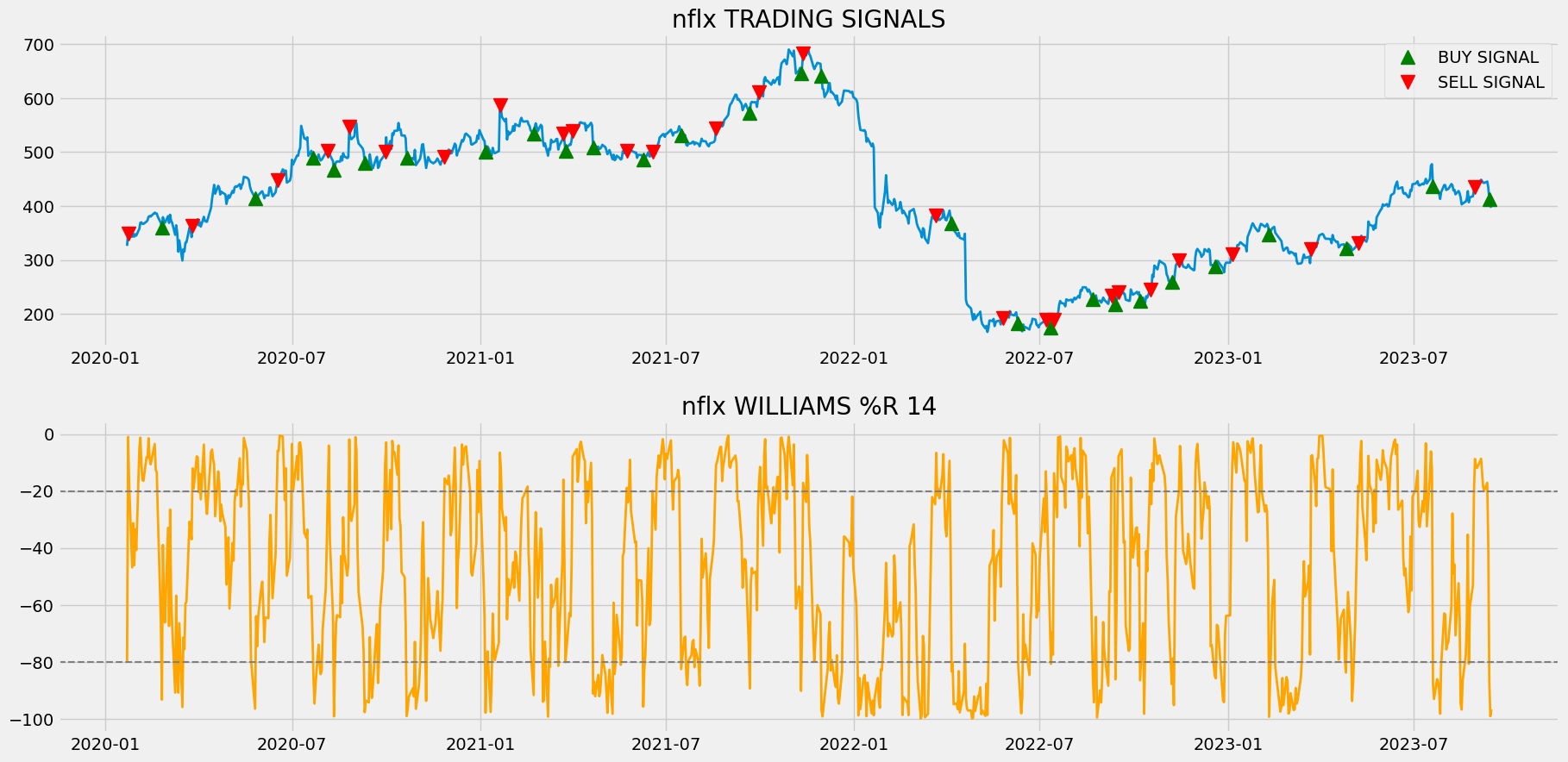
Code Explanation: We are plotting the readings of Williams %R along with the buy and sell signals generated by the trading strategy. We can observe that whenever the Williams %R line crosses from below to above -20 and, a green-colored buy signal is plotted in the chart. Similarly, whenever the Williams %R line crosses from above to below -80 and, a red-colored sell signal is plotted in the chart.

Step-7: Creating our Position

In this step, we are going to create a list that indicates 1 if we hold the stock or 0 if we don’t own or hold the stock.

Python Implementation:

position = []
for i in range(len(wr_signal)):
    if wr_signal[i] > 1:
        position.append(0)
    else:
        position.append(1)
        
for i in range(len(nflx['close'])):
    if wr_signal[i] == 1:
        position[i] = 1
    elif wr_signal[i] == -1:
        position[i] = 0
    else:
        position[i] = position[i-1]
        
close_price = nflx['close']
wr = nflx['wr_14']
wr_signal = pd.DataFrame(wr_signal).rename(columns = {0:'wr_signal'}).set_index(nflx.index)
position = pd.DataFrame(position).rename(columns = {0:'wr_position'}).set_index(nflx.index)

frames = [close_price, wr, wr_signal, position]
strategy = pd.concat(frames, join = 'inner', axis = 1)

strategy.head()

Output:

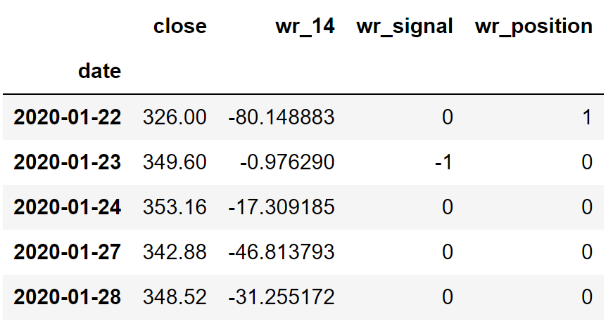
Code Explanation: First, we are creating an empty list named ‘position’. We are passing two for-loops, one is to generate values for the ‘position’ list to just match the length of the ‘signal’ list. The other for-loop is the one we are using to generate actual position values. Inside the second for-loop, we are iterating over the values of the ‘signal’ list, and the values of the ‘position’ list get appended concerning which condition gets satisfied. The value of the position remains 1 if we hold the stock or remains 0 if we sold or don’t own the stock. Finally, we are doing some data manipulations to combine all the created lists into one dataframe.

From the output being shown, we can see that in the first row our position in the stock has remained 1 (since there isn’t any change in the Williams %R signal) but our position suddenly turned to -1 as we sold the stock when the Williams %R trading signal represents a sell signal (-1). Our position will remain 0 until some changes in the trading signal occur. Now it’s time to do implement some backtesting process!

Step-8: Backtesting

Before moving on, it is essential to know what backtesting is. Backtesting is the process of seeing how well our trading strategy has performed on the given stock data. In our case, we are going to implement a backtesting process for our Williams %R trading strategy over the Netflix stock data.

Python Implementation:

nflx_ret = pd.DataFrame(np.diff(nflx['close'])).rename(columns = {0:'returns'})
wr_strategy_ret = []

for i in range(len(nflx_ret)):
    returns = nflx_ret['returns'][i]*strategy['wr_position'][i]
    wr_strategy_ret.append(returns)
    
wr_strategy_ret_df = pd.DataFrame(wr_strategy_ret).rename(columns = {0:'wr_returns'})
investment_value = 100000
wr_investment_ret = []

for i in range(len(wr_strategy_ret_df['wr_returns'])):
    number_of_stocks = floor(investment_value/nflx['close'][i])
    returns = number_of_stocks*wr_strategy_ret_df['wr_returns'][i]
    wr_investment_ret.append(returns)

wr_investment_ret_df = pd.DataFrame(wr_investment_ret).rename(columns = {0:'investment_returns'})
total_investment_ret = round(sum(wr_investment_ret_df['investment_returns']), 2)
profit_percentage = floor((total_investment_ret/investment_value)*100)
print(cl('Profit gained from the W%R strategy by investing $100k in NFLX : {}'.format(total_investment_ret), attrs = ['bold']))
print(cl('Profit percentage of the W%R strategy : {}%'.format(profit_percentage), attrs = ['bold']))

Output:

Profit gained from the W%R strategy by investing $100k in NFLX : 57772.45
Profit percentage of the W%R strategy : 57%

Code Explanation: First, we are calculating the returns of the Netflix stock using the ‘diff’ function provided by the NumPy package and we have stored it as a dataframe into the ‘nflx_ret’ variable. Next, we are passing a for-loop to iterate over the values of the ‘nflx_ret’ variable to calculate the returns we gained from our Williams %R trading strategy, and these returns values are appended to the ‘wr_strategy_ret’ list. Next, we are converting the ‘wr_strategy_ret’ list into a dataframe and stored it into the ‘wr_strategy_ret_df’ variable.

Next comes the backtesting process. We are going to backtest our strategy by investing a hundred thousand USD into our trading strategy. So first, we are storing the amount of investment into the ‘investment_value’ variable. After that, we are calculating the number of Netflix stocks we can buy using the investment amount. You can notice that I’ve used the ‘floor’ function provided by the Math package because, while dividing the investment amount by the closing price of Netflix stock, it spits out an output with decimal numbers. The number of stocks should be an integer but not a decimal number. Using the ‘floor’ function, we can cut out the decimals. Remember that the ‘floor’ function is way more complex than the ‘round’ function. Then, we are passing a for-loop to find the investment returns followed by some data manipulation tasks.

Finally, we are printing the total return we got by investing a hundred thousand into our trading strategy and it is revealed that we have made an approximate profit of fifty-seven thousand USD in one year. That’s not bad! Now, let’s compare our returns with SPY ETF (an ETF designed to track the S&P 500 stock market index) returns.

Step-9: SPY ETF Comparison

This step is optional but it is highly recommended as we can get an idea of how well our trading strategy performs against a benchmark (SPY ETF). In this step, we are going to extract the data of the SPY ETF using the ‘get_historical_data’ function we created and compare the returns we get from the SPY ETF with our Williams %R trading strategy returns on Netflix.

Python Implementation:

def get_benchmark(start_date, investment_value):
    spy = get_historical_data('SPY', start_date)['close']
    benchmark = pd.DataFrame(np.diff(spy)).rename(columns = {0:'benchmark_returns'})
    
    investment_value = investment_value
    benchmark_investment_ret = []
    
    for i in range(len(benchmark['benchmark_returns'])):
        number_of_stocks = floor(investment_value/spy[i])
        returns = number_of_stocks*benchmark['benchmark_returns'][i]
        benchmark_investment_ret.append(returns)

    benchmark_investment_ret_df = pd.DataFrame(benchmark_investment_ret).rename(columns = {0:'investment_returns'})
    return benchmark_investment_ret_df

benchmark = get_benchmark('2020-01-01', 100000)

investment_value = 100000
total_benchmark_investment_ret = round(sum(benchmark['investment_returns']), 2)
benchmark_profit_percentage = floor((total_benchmark_investment_ret/investment_value)*100)
print(cl('Benchmark profit by investing $100k : {}'.format(total_benchmark_investment_ret), attrs = ['bold']))
print(cl('Benchmark Profit percentage : {}%'.format(benchmark_profit_percentage), attrs = ['bold']))
print(cl('W%R Strategy profit is {}% higher than the Benchmark Profit'.format(profit_percentage - benchmark_profit_percentage), attrs = ['bold']))

Output:

Benchmark profit by investing $100k : 22431.5
Benchmark Profit percentage : 22%
W%R Strategy profit is 35% higher than the Benchmark Profit

Code Explanation: The code used in this step is almost similar to the one used in the previous backtesting step but, instead of investing in Netflix, we are investing in SPY ETF by not implementing any trading strategies. From the output, we can see that our Williams %R trading strategy has outperformed the SPY ETF by 35%. That’s great!

Final Thoughts!

After a long process of crushing both theory and coding parts on Williams %R, we have successfully built a profitable trading strategy that exceeds the returns of SPY ETF. That’s great but, that isn’t enough. When I ran a separate backtest process to gain more insights on the performance of our trading strategy, I came to know that our Williams %R-based strategy returns are less than that of the actual Netflix stock return. The foremost reason behind this might be strategy optimization.

What is strategy optimization? It is the process of tuning a trading strategy to perform to its best. The best way to tune a strategy, especially a leading indicator trading strategy is to add another technical indicator as a filter. This filter acts as a gauge to ensure that the trading signals being revealed by the strategy are authentic but not false. This part should be considered essential while using Williams %R since this indicator is prone to revealing many false signals which ultimately ends up resulting in us making bad trades. Coming back to strategy optimization, it is not only about adding another technical indicator but also includes efficient risk management steps, and a better trading environment.

If you manage to achieve these things, you will have a robust trading algorithm in your hand that is ready to make some better trades in the real-world market. So I highly recommend you to try these things out. You might question me on why I haven’t touched upon these topics in the article because the sole incentive of the article is not to encourage people to create profitable trading strategies and mint money from the market but to educate people about a powerful trading indicator. That’s it! You’ve reached the end of the article. Hope you learned something new and useful from this article.

Williams %R

Implementation in Python

Step-1: Importing Packages

Step-2: API Key Activation

Step-3: Extracting Historical Data

Step-3: Williams %R Calculation

Step-4: Williams %R Plot

Step-5: Creating the trading strategy

Step-6: Plotting the trading signals

Step-7: Creating our Position

Step-8: Backtesting

Step-9: SPY ETF Comparison

Final Thoughts!

Related Articles

Backtesting Technical Analysis Strategies with Excel(SMA, RSI, MACD)

Using Delisted Stocks for Backtesting a 3-EMA Strategy with Python

Practical Guide to Automated Detection Trading Patterns with Python

Benchmark Tracking and Cointegration Analysis with Python

Backtesting a Killer Mean Reversion Trading Strategy with Python

Maximising Profits Trading with Moving Average Crossovers