
Every technical indicator out there is simply great and unique in its own perspective and usage. But most of them never fail to fall into one and the same pitfall – which is the ranging markets. What is a ranging market? Ranging markets are markets that show no trend or momentum but move back and forth between specific high and low price ranges (these markets are also called choppy, sideways, and flat markets). Technical indicators are prone to revealing false entry and exit points while markets are ranging. Fortunately, we have a set of indicators that are designed particularly to observe whether a market is ranging or not. Such indicators are called volatility indicators.
There are a lot of them that come under this category, but the one that dominates the game is the Choppiness Index. In this article, we will first understand the concept of the Choppiness Index and how it’s being calculated and then code the indicator from scratch in Python. We will also discuss how to use the Choppiness Index to detect ranging and trending periods in a market.
Quick jump:
Volatility and ATR
Before jumping on to exploring the Choppiness Index, it is essential to have some basic idea of two important concepts: Volatility and Average True Range (ATR). Volatility is the measure of the magnitude of price variation or dispersion. The higher the volatility, the higher the risk, and vice-versa. People having expertise in this concept will have the possibility to hold a tremendous edge in the market. We have tons of tools to calculate the Volatility of a market, but none can achieve a hundred percent accuracy in measuring it; however, there are some that have the potential to calculate with more accuracy. One such tool is the Average True Range, shortly known as ATR.
Founded by Wilder Wiles, the Average True Range is a technical indicator that measures how much an asset moves on average. It is a lagging indicator meaning that it takes into account the historical data of an asset to measure the current value but it’s not capable of predicting the future data points. This is not considered as a drawback while using ATR as it’s one of the indicators to track the volatility of a market more accurately. Along with being a lagging indicator, ATR is also a non-directional indicator meaning that the movement of ATR is inversely proportional to the actual movement of the market. To calculate ATR, it is requisite to follow two steps:
- Calculate True Range (TR): A True Range of an asset is calculated by taking the greatest values of three price differences which are: market high minus market low, market high minus previous market close, and previous market close minus market low. It can be represented as follows:
MAX [ {HIGH - LOW}, {HIGH - P.CLOSE}, {P.CLOSE - LOW} ]

where,
MAX = Maximum values
HIGH = Market High
LOW = Market Low
P.CLOSE = Previous market close
- Calculate ATR: The calculation for the Average True Range is simple. We just have to take a smoothed average of the previously calculated True Range values for a specified number of periods. The smoothed average is not just any SMA or EMA but an own type of smoothed average created by Wilder Wiles himself but there aren’t any restrictions in using other MAs too. In this article, we will be using SMA rather than the custom moving average created by the founder of the indicator to make things simple. The calculation of ATR with a traditional setting of 14 as the number of periods can be represented as follows:
ATR 14 = SMA 14 [ TR ]

where,
ATR 14 = 14 Period Average True Range
SMA 14 = 14 Period Simple Moving Average
TR = True Range
While using ATR as an indicator for trading purposes, traders must ensure that they are more cautious than ever, as the indicator is very lagging. Now that we have an understanding of what volatility and Average True Range are, let’s dive into the main concept of this article: the Choppiness Index.
Choppiness Index
The Choppiness Index is a volatility indicator that is used to identify whether a market is ranging or trending. The characteristics of the Choppiness Index are almost similar to ATR. It is a lagging and non-directional indicator whose values rise when the market is bound to consolidate and decrease in value when the market shows high momentum or price actions. The calculation of the Choppiness Index involves two steps:
- ATR calculation: In this step, the ATR of an asset is calculated with one as the specified number of periods.
- Choppiness Index calculation: To calculate the Choppiness Index with a traditional setting of 14 as the lookback period is calculated by first taking log 10 of the value received by dividing the 14-day total of the previously calculated ATR 1 by the difference between the 14-day highest high and 14-day lowest low. This value is then divided by log 10 of the lookback period and finally multiplied by 100. This might sound confusing but will be easy to understand once you see the representation of the calculation:
CI14 = 100 * LOG10 [14D ATR1 SUM/(14D HIGHH - 14D LOWL)] / LOG10(14)

where,
CI14 = 14-day Choppiness Index
14D ATR1 SUM = 14-day sum of ATR with 1 as lookback period
14D HIGHH = 14-day highest high
14D LOWL - 14-day lowest low
This concludes our theory part on the Choppiness Index. Now let’s code the indicator from scratch in Python. Before moving on, a note on disclaimer: This article’s sole purpose is to educate people and must be considered as an information piece but not as investment advice or so.
Implementation in Python
Our process starts with importing the essential packages into our Python environment. Then, we will be pulling the historical stock data of Tesla using the eod Python package provided by EOD Historical Data (EODHD). After that, we will build the Choppiness Index from scratch.
Step-1: Importing Packages
Importing the required packages into the Python environment is a non-skippable step. The primary packages are going to be eodhd for extracting historical stock data, Pandas for data formatting and manipulations, NumPy to work with arrays and for complex functions, and Matplotlib for plotting purposes. The secondary packages are going to be Math for mathematical functions and Termcolor for font customization (optional).
Python Implementation:
# IMPORTING PACKAGES

import numpy as np
import matplotlib.pyplot as plt
import pandas as pd
from termcolor import colored as cl
from math import floor
from eodhd import APIClient

plt.rcParams['figure.figsize'] = (20,10)
plt.style.use('fivethirtyeight')
With the required packages imported into Python, we can proceed to fetch historical data for Tesla using EODHD’s eodhd Python library. Also, if you haven’t installed any of the imported packages, make sure to do so using the pip command in your terminal.
Step-2: API Key Activation
It is essential to register the EODHD API key with the package in order to use its functions. If you don’t have an EODHD API key, firstly, head over to their website, then, finish the registration process to create an EODHD account, and finally, navigate to the ‘Settings’ page where you could find your secret EODHD API key. It is important to ensure that this secret API key is not revealed to anyone. You can activate the API key by following this code:
api_key = '<YOUR API KEY>'
client = APIClient(api_key)
The code is pretty simple. In the first line, we are storing the secret EODHD API key into the api_key and then in the second line, we are using the APIClient class provided by the eodhd package to activate the API key and stored the response in the client variable.
Note that you need to replace <YOUR API KEY> with your secret EODHD API key. Apart from directly storing the API key with text, there are other ways for better security such as utilizing environmental variables, and so on.
Step-3: Extracting Historical Data
Before heading into the extraction part, it is first essential to have some background about historical or end-of-day data. In a nutshell, historical data consists of information accumulated over a period of time. It helps in identifying patterns and trends in the data. It also assists in studying market behavior. Now, you can easily extract the historical data of any tradeable assets using the eod package by following this code:
# EXTRACTING HISTORICAL DATA
def get_historical_data(ticker, start_date):
json_resp = client.get_eod_historical_stock_market_data(symbol = ticker, period = 'd', from_date = start_date, order = 'a')
df = pd.DataFrame(json_resp)
df = df.set_index('date')
df.index = pd.to_datetime(df.index)
return df
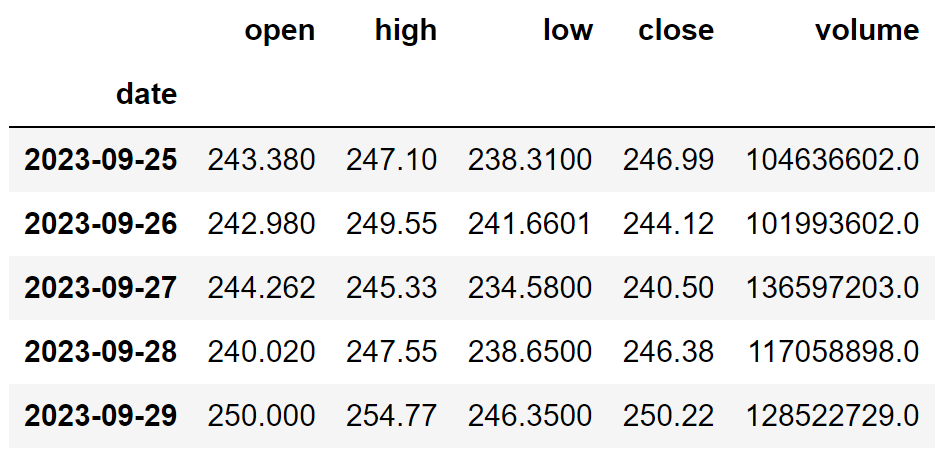
tsla = get_historical_data('TSLA', '2020-01-01')
tsla.tail()In the above code, we are using the get_eod_historical_stock_market_data function provided by the eodhd package to extract the split-adjusted historical stock data of Tesla. The function consists of the following parameters:
- the
tickerparameter where the symbol of the stock we are interested in extracting the data should be mentioned - the
periodrefers to the time interval between each data point (one-day interval in our case). - the
from_dateandto_dateparameters which indicate the starting and ending date of the data respectively. The format of the input should be “YYYY-MM-DD” - the
orderparameter which is an optional parameter that can be used to order the dataframe either in ascending (a) or descending (d). It is ordered based on the dates.
After extracting the historical data, we are performing some data-wrangling processes to clean and format the data. The final dataframe looks like this:
Step-3: Choppiness Index Calculation
In this step, we are going to calculate the values of the Choppiness Index with 14 as the lookback period using the Choppiness Index formula we discussed before.
Python Implementation:
def get_ci(high, low, close, lookback):
tr1 = pd.DataFrame(high - low).rename(columns = {0:'tr1'})
tr2 = pd.DataFrame(abs(high - close.shift(1))).rename(columns = {0:'tr2'})
tr3 = pd.DataFrame(abs(low - close.shift(1))).rename(columns = {0:'tr3'})
frames = [tr1, tr2, tr3]
tr = pd.concat(frames, axis = 1, join = 'inner').dropna().max(axis = 1)
atr = tr.rolling(1).mean()
highh = high.rolling(lookback).max()
lowl = low.rolling(lookback).min()
ci = 100 * np.log10((atr.rolling(lookback).sum()) / (highh - lowl)) / np.log10(lookback)
return ci
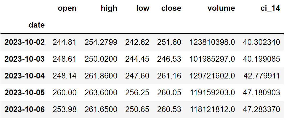
tsla['ci_14'] = get_ci(tsla['high'], tsla['low'], tsla['close'], 14)
tsla = tsla.dropna()
tsla.tail()Output:
Code Explanation: First we are defining a function named ‘get_ci’ that takes the stock’s high price data (‘high’), low price data (‘low’), close price data (‘close’), and the lookback period as parameters.
Inside the function, we are first finding the three differences that are essential for the calculation of True Range. To calculate TR, we are picking the maximum values from those three differences using the ‘max’ function provided by the Pandas package. With the lookback period as 1, we are taking the SMA of TR using the ‘rolling’ and ‘mean’ function to calculate the Average True Index and stored the values into the ‘atr’ variable. Next, we are defining two variables ‘highh’ and ‘lowl’ to store the highest high and lowest low of the stock for a specified lookback period. Now, we are substituting all the calculated values into the formula we discussed before to get the values of the Choppiness Index.
Finally, we are calling the defined function to get the Choppiness Index values of Tesla with the traditional lookback period of 14.
Using Choppiness Index
The values of the Choppiness Index bound between 0 to 100, hence acting as a range-bound oscillator. The closer the values фку to 100, the higher the choppiness, and vice-versa. Usually, two levels are constructed above and below the Choppiness Index plot which is used to identify whether a market is ranging or trending. The above level is usually plotted at a higher threshold of 61.8 and if the values of the Choppiness Index are equal to or above this threshold, then the market is considered to be ranging or consolidating. Likewise, the below level is plotted at a lower threshold of 38.2 and if the Choppiness Index has a reading of or below this threshold, then the market is considered to be trending. The usage of the Choppiness Index can be represented as follows:
IF CHOPPINESS INDEX >= 61.8 --> MARKET IS CONSOLIDATING
IF CHOPPINESS INDEX <= 38.2 --> MARKET IS TRENDING
Now let’s use the Choppiness Index to identify the ranging and trending market periods of Tesla by plotting the calculated values in python.
Python Implementation:
ax1 = plt.subplot2grid((11,1,), (0,0), rowspan = 5, colspan = 1)
ax2 = plt.subplot2grid((11,1,), (6,0), rowspan = 4, colspan = 1)
ax1.plot(tsla['close'], linewidth = 2.5, color = '#2196f3')
ax1.set_title('TSLA CLOSING PRICES')
ax2.plot(tsla['ci_14'], linewidth = 2.5, color = '#fb8c00')
ax2.axhline(38.2, linestyle = '--', linewidth = 1.5, color = 'grey')
ax2.axhline(61.8, linestyle = '--', linewidth = 1.5, color = 'grey')
ax2.set_title('TSLA CHOPPINESS INDEX 14')
plt.show()
Output:
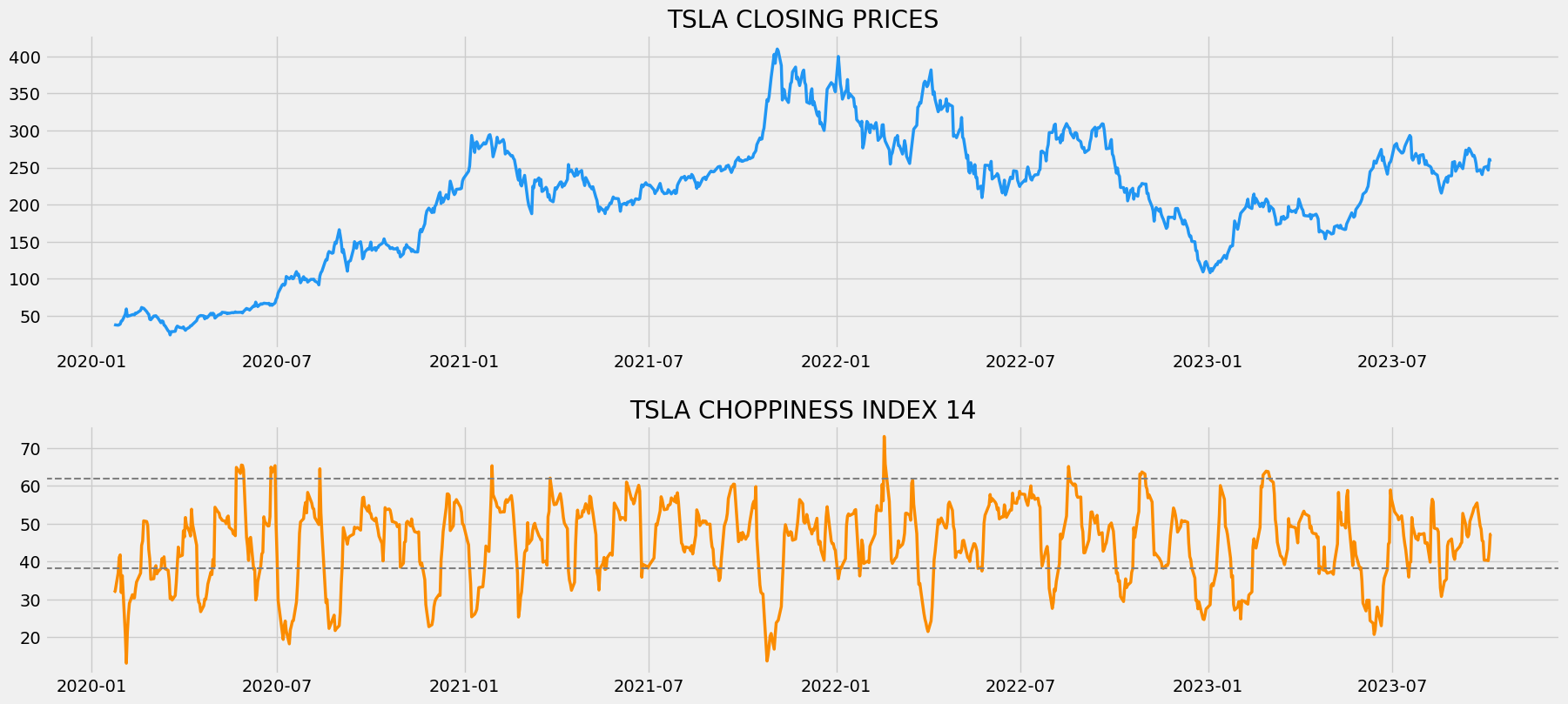
The above chart is separated into two panels: the above panel with the closing price of Tesla and the lower panel with the values of the 14-day Choppiness Index of Tesla. As you can see, there are two lines plotted above and below the Choppiness Index plot which represents the two thresholds used to identify the market movement. Tesla, being a volatile stock with higher price movements, has frequent readings below the lower threshold of 38.2. This means, that Tesla shows huge momentum with higher volatility. We can confirm the readings of the Choppiness Index by seeing the actual price movements parallelly. Likewise, in some places, the Choppiness Index readings exceed the higher threshold of 61.8, representing that the stock is consolidating. This is the traditional and the right way to use the Choppiness Index in the real-world market.
Final Thoughts!
After a long process of theory and coding, we have successfully gained some understanding of what the Choppiness Index is all about and its calculation and usage. It might seem to be a simple indicator but it’s very useful while trading and saves you from depleting your capital. Since the Choppiness Index is very lagging, ensure that you’re more cautious than ever while using it for trading purposes. Also, you should not completely rely just on the Choppiness Index for generating entry and exit points but can be used as a filter for your actual trading strategy. There are two things to remember while using the Choppiness Index in the real-world market:
- Strategy Optimization: The Choppiness Index is not just about the higher and lower threshold but it has the potential to be more. So, before entering the real-world market, make sure that you have a robust and optimized trading strategy that uses the Choppiness Index as a filter.
- Backtesting: Drawing conclusions by just backtesting the algorithm in one asset or so won’t be effective and sometimes can even lead to unexpected turns. The real-world market doesn’t work the same every time. In order to make better trades, try backtesting the trading strategy with different assets and modify the strategy if needed.
That’s it! Hope you learned something useful from this article. Happy learning!