People who are in the field of stock trading will most certainly know about the Stochastic Oscillator given its popularity, and today we are going to explore an indicator that is not only similar but also performs like the Stochastic Oscillator too. It’s the Relative Vigor Index, shortly known as RVI. In this article, we will first build some basic intuitions about the indicator and the mathematics behind it. Then we will proceed to the programming where we will use Python to build the indicator from scratch, backtest a trading strategy based on it, and compare the strategy results with those of SPY ETF (an ETF specifically designed to track the movement of the S&P 500 market index). Without further ado, let’s dive into the article.

Quick jump:

1 Relative Vigor Index (RVI)
- 1.1 RVI line calculation
- 1.2 Signal line calculation
2 Implementation in Python
3 Final Thoughts!

Relative Vigor Index (RVI)

The Relative Vigor Index is a momentum indicator that acts as an instrument to determine the current market momentum, either upward or downward. Unlike the Stochastic Oscillator, the Relative Vigor Index is an unbounded oscillator and does not fluctuate between certain thresholds rather it oscillates across a center-line (zero in most cases). The Relative Vigor Index is composed of two components: the RVI line and the Signal line. Now let’s see how each of the components is being calculated.

RVI line calculation

To calculate the readings of the RVI line, we must first determine the numerator and the denominator.

The numerator can be calculated in five steps:

Find the difference between the current closing price and the current opening price of a stock. We’ll name the difference ‘a’.
Find the difference between the closing price two periods ago and the opening price two periods ago, this difference is multiplied by 2. We’ll name the result ‘b’.
Find the difference between the closing price three periods ago and the opening price three periods, then multiplied them two. We’ll name the result ‘c’.
Multiply the difference that we get by subtracting the opening price four periods ago from the closing price four periods ago by two, and the result will be named ‘d’.
The final step is to add the determined a, b, c, and d variables to each other and a rolling sum for a specified number of periods is calculated (a typical setting is 4). The numerator calculation can be represented as follows:

a = CURRENT CLOSE - CURRENT OPEN
b =  2 * ( CLOSE 2 PERIODS AGO - OPEN 2 PERIODS AGO )
c =  2 * ( CLOSE 3 PERIODS AGO - OPEN 3 PERIODS AGO )
d =  2 * ( CLOSE 4 PERIODS AGO - OPEN 4 PERIODS AGO )
Numerator = ROLLING SUM 4 [ a + b + c + d ]

The procedure to calculate the denominator is almost similar to that of the numerator, but we just have to replace the closing price and the opening price data with high and low price data respectively.

The denominator can be calculated in five steps:

Find the difference between the current high price and the current low price of a stock. We’ll name the difference ‘e’.
Find the difference between the high price two periods ago and the low price two periods ago, and this difference is multiplied by 2. We’ll name the result ‘f’.
Find the difference between the high price three periods ago and the low price three periods, then multiply it by two. We’ll name the result ‘g’.
Multiply the difference that we get by subtracting the low price four periods ago from the high price four periods ago by two, and we’ll name the result ‘h’.
The final step is to add the determined e, f, g, and h variables to each other and a rolling sum with 4 as the lookback period is calculated. The denominator calculation can be represented as follows:

e = CURRENT HIGH - CURRENT LOW
f =  2 * ( HIGH 2 PERIODS AGO - LOW 2 PERIODS AGO )
g =  2 * ( HIGH 3 PERIODS AGO - LOW 3 PERIODS AGO )
h =  2 * ( HIGH 4 PERIODS AGO - LOW 4 PERIODS AGO )
Denominator = ROLLING SUM 4 [ e + f + g + h ]

After getting the numerator and the denominator, we can move on to calculating the readings of the RVI line: divide the numerator by the denominator, and the result is smoothed by a Simple Moving Average for a specified number of lookback periods (typically 10). The calculation can be mathematically represented as follows:

RVI LINE = SMA 10 [ NUMERATOR / DENOMINATOR ]

Signal line calculation

Usually, the indicators having the signal line as a component are calculated by taking either Simple Moving Average or Exponential Moving Average of the main component (RVI line in our case) for a specified number of periods. But it’s different with the Relative Vigor Index.

There are four main steps involved in the calculation of the Signal line:

The first step is to multiply the RVI line readings one period with two. We’ll call this ‘rvi1’.
The next step is to multiply the readings of the RVI line two periods ago with two. We’ll call this ‘rvi2’.
The third step is to determine the RVI line readings three periods ago, we’ll call this ‘rvi3’.
The final step is to add the determined ‘rvi1’, ‘rvi2’, ‘rvi3’ along with the readings of the RVI line to each other, and the total sum or the result is divided by 6. The calculation can be represented as follows:

rvi1 = 2 * RVI LINE 1 PERIOD AGO
rvi2 = 2 * RVI LINE 2 PERIODS AGO
rvi3 = RVI LINE 3 PERIODS AGO
SIGNAL LINE = ( RVI LINE + rvi1 + rvi2 + rvi3 ) / 6

That’s the whole process of calculating the components of the Relative Vigor Index.

Now let’s analyze a chart where Apple’s closing price data is plotted along with its Relative Vigor Index calculated with 10 as the lookback period to build a solid understanding of the indicator and how it’s being used.

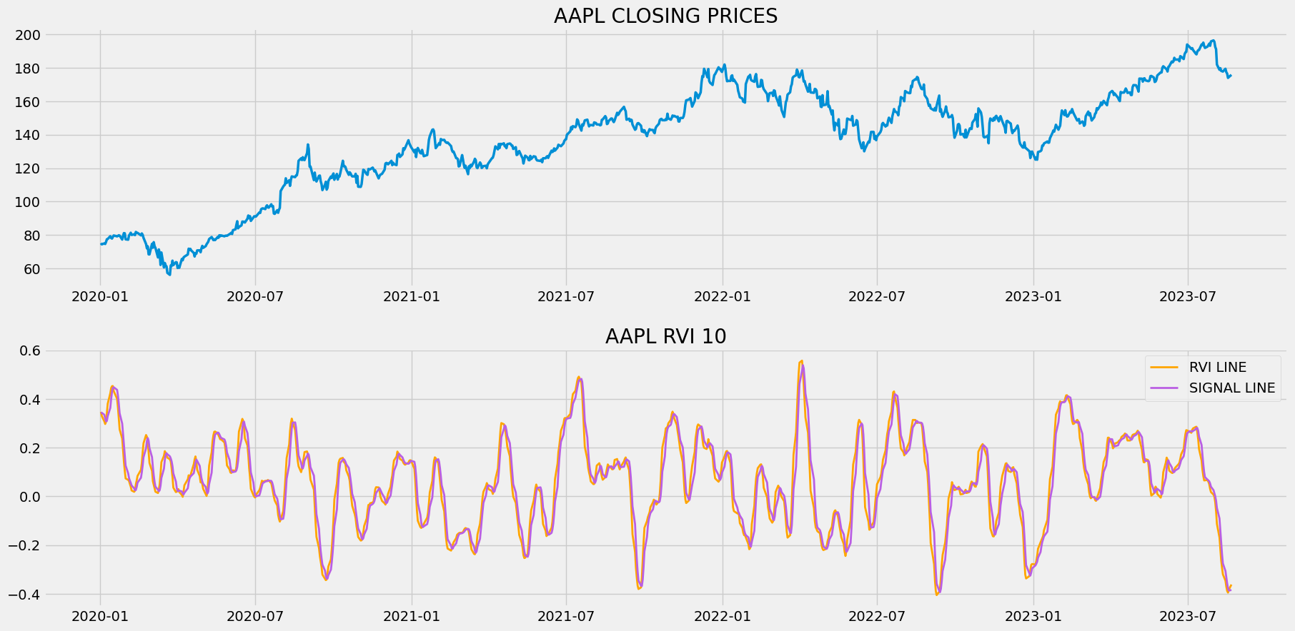
The above chart is separated into two panels: the upper panel with the plot of Apple’s closing price data, and the lower panel with the components of the Relative Vigor Index calculated with 10 as the lookback period. The main characteristic feature of the indicator is to help traders with identifying the current market momentum and this can be seen clearly in the chart where the components of the RVI indicator rises positively when the market shows a sturdy upward momentum, and decreases when the market is in the state of strong downward momentum. As I said before, the Relative Vigor Index is an unbounded oscillator and the above chart proves this statement where it can be seen that the components of the RVI indicator do not fluctuate between certain upper and lower thresholds like other momentum oscillators but instead, across the zero-line or the center-line.

Speaking about trading strategies, to my knowledge, it is possible to apply three types of trading strategies based on the Relative Vigor Index. The first is the divergence trading strategy, the second one is the classic crossover strategy, and the third one is the overbought and oversold strategy. In this article, we are going to implement the second type of trading strategy – the crossover strategy. This strategy reveals a buy signal whenever the RVI line crosses from below to above the Signal line, and similarly, reveals a sell signal whenever the RVI line goes from above to below the Signal line. The RVI crossover trading strategy can be represented as follows:

IF PREV.RLINE < PREV.SLINE AND CUR.RLINE > CUR.SLINE ==> BUY SIGNAL
IF PREV.RLINE > PREV.SLINE AND CUR.RLINE < CUR.SLINE ==> SELL SIGNAL

In most cases, traders use the Relative Vigor Index accompanied by another technical indicator to build a trading strategy but that is not the scope of this article (recommended to try doing). That’s it! This concludes our theory part on the Relative Vigor Index and let’s move on to the programming part where we will use Python to first build the indicator from scratch, construct the crossover trading strategy, backtest the strategy on Apple stock data, and finally compare the results with that of SPY ETF. Let’s do some coding! Before moving on, a note on disclaimer: This article’s sole purpose is to educate people and must be considered as an information piece but not as investment advice.

Implementation in Python

The coding part is classified into various steps as follows:

1. Importing Packages
2. Extracting Stock Data from EODHD
3. Relative Vigor Index Calculation
4. Creating the Crossover Trading Strategy
5. Plotting the Trading Lists
6. Creating our Position
7. Backtesting
8. SPY ETF Comparison

We will be following the order mentioned in the above list, so buckle up your seatbelts to follow every upcoming coding part.

Step-1: Importing Packages

Importing the required packages into the Python environment is a non-skippable step. The primary packages are going to be Pandas to work with data, NumPy to work with arrays and for complex functions, Matplotlib for plotting purposes, and Requests to make API calls. The secondary packages are going to be Math for mathematical functions and Termcolor for font customization (optional).

Python Implementation:

# IMPORTING PACKAGES

import pandas as pd
import matplotlib.pyplot as plt
import numpy as np
import requests
from termcolor import colored as cl
from math import floor

plt.style.use('fivethirtyeight')
plt.rcParams['figure.figsize'] = (20,10)

With the required packages imported into Python, we can proceed to fetch historical data for Apple using EODHD’s OHLC split-adjusted data API endpoint.

Step-2: Extracting data from EODHD

In this phase, we’re set to retrieve the historical stock data for Apple using the OHLC split-adjusted API endpoint provided by EODHD. It’s important to note that EOD Historical Data (EODHD) is a reliable provider of financial APIs, encompassing an extensive array of market data, including historical data and economic news. Be sure to possess an EODHD account and access your secret API key, a crucial element for data extraction via the API.

Python Implementation:

# EXTRACTING STOCK DATA

def get_historical_data(symbol, start_date):
    api_key = 'YOUR API KEY'
    api_url = f'https://eodhistoricaldata.com/api/technical/{symbol}?order=a&fmt=json&from={start_date}&function=splitadjusted&api_token={api_key}'
    raw_df = requests.get(api_url).json()
    df = pd.DataFrame(raw_df)
    df.date = pd.to_datetime(df.date)
    df = df.set_index('date')
    return df

aapl = get_historical_data('AAPL', '2019-01-01')
aapl.tail()

Output:

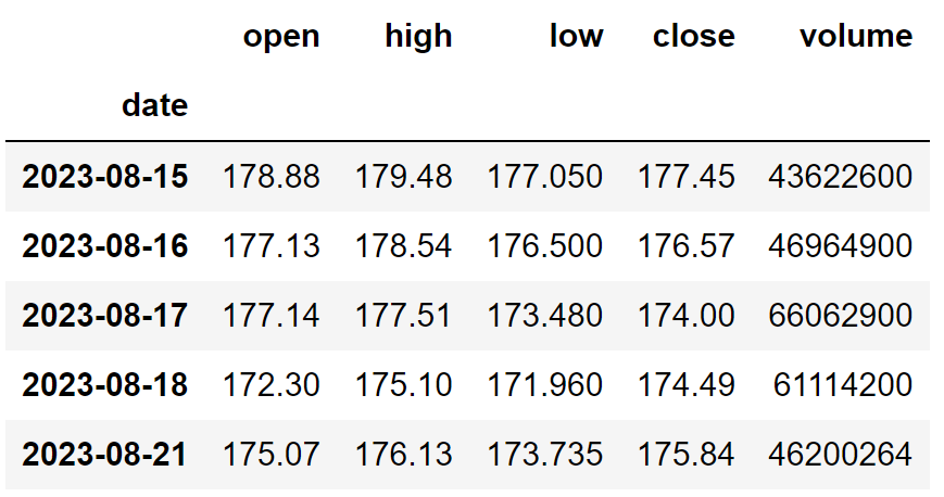
Code Explanation: We begin by defining a function named ‘get_historical_data,’ which takes the stock symbol (‘symbol’) and the start date for historical data (‘start_date’) as parameters. Inside the function, we define the API key and URL, then retrieve the historical data in JSON format using the ‘get’ function and store it in the ‘raw_df’ variable. After cleaning and formatting the raw JSON data, we return it as a Pandas dataframe. Finally, we call this function to fetch Apple’s historical data from the start of 2019 and store it in the ‘aapl’ variable.

Step-3: Relative Vigor Index Calculation

In this step, we are going to calculate the components of the Relative Vigor Index by following the methods and formulas we discussed before.

Python Implementation:

# RELATIVE VIGOR INDEX CALCULATION

def get_rvi(open, high, low, close, lookback):
    a = close - open
    b = 2 * (close.shift(2) - open.shift(2))
    c = 2 * (close.shift(3) - open.shift(3))
    d = close.shift(4) - open.shift(4)
    numerator = a + b + c + d
    
    e = high - low
    f = 2 * (high.shift(2) - low.shift(2))
    g = 2 * (high.shift(3) - low.shift(3))
    h = high.shift(4) - low.shift(4)
    denominator = e + f + g + h
    
    numerator_sum = numerator.rolling(4).sum()
    denominator_sum = denominator.rolling(4).sum()
    rvi = (numerator_sum / denominator_sum).rolling(lookback).mean()
    
    rvi1 = 2 * rvi.shift(1)
    rvi2 = 2 * rvi.shift(2)
    rvi3 = rvi.shift(3)
    rvi_signal = (rvi + rvi1 + rvi2 + rvi3) / 6
    
    return rvi, rvi_signal

aapl['rvi'], aapl['signal_line'] = get_rvi(aapl['open'], aapl['high'], aapl['low'], aapl['close'], 10)
aapl = aapl.dropna()
aapl = aapl[aapl.index >= '2020-01-01']
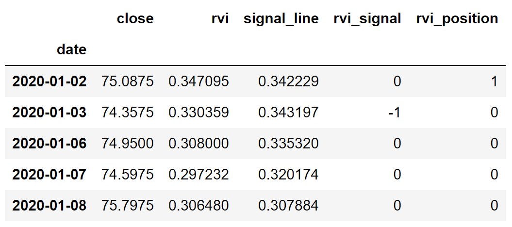
aapl.tail()

Output:

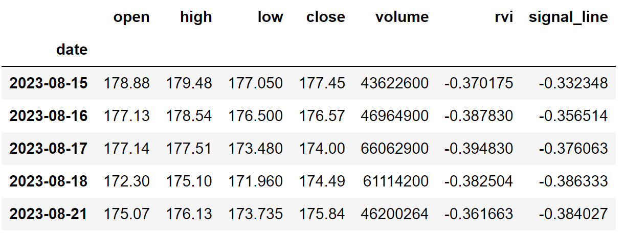
Code Explanation: We are first defining a function named ‘get_rvi’ that takes a stock’s opening (‘open’), high (‘high’), low (‘low’), closing (‘close’) price data, and the lookback period (‘lookback’) as parameters.

Inside the function, we are first calculating the variables involved in the calculation of the numerator which is a, b, c, and d. These are variables are calculated by following the formulas we discussed before and added to each other to determine the numerator. Next comes the calculation of the denominator that is almost similar to that of the numerator calculation but we are just replacing certain values. Before calculating the readings of the RVI line, we are determining the rolling sum of both the numerator and denominator with 4 as the lookback period and the results are then substituted into the formula of the RVI line to get the readings.

After that, we are calculating the three prerequisite variables which are rvi1, rvi2, and rvi3 we discussed before, and substituting into the formula of the Signal line along with the previously calculated RVI line values to get the readings. Finally, we are returning and calling the function the store Apple’s Relative Vigor Index readings with 10 as the lookback period.

Step-4: Creating the trading strategy

In this step, we are going to implement the discussed Relative Vigor Index crossover trading strategy in Python.

Python Implementation:

# RELATIVE VIGOR INDEX STRATEGY

def implement_rvi_strategy(prices, rvi, signal_line):
    buy_price = []
    sell_price = []
    rvi_signal = []
    signal = 0
    
    for i in range(len(prices)):
        if rvi[i-1] < signal_line[i-1] and rvi[i] > signal_line[i]:
            if signal != 1:
                buy_price.append(prices[i])
                sell_price.append(np.nan)
                signal = 1
                rvi_signal.append(signal)
            else:
                buy_price.append(np.nan)
                sell_price.append(np.nan)
                rvi_signal.append(0)
        elif rvi[i-1] > signal_line[i-1] and rvi[i] < signal_line[i]:
            if signal != -1:
                buy_price.append(np.nan)
                sell_price.append(prices[i])
                signal = -1
                rvi_signal.append(signal)
            else:
                buy_price.append(np.nan)
                sell_price.append(np.nan)
                rvi_signal.append(0)
        else:
            buy_price.append(np.nan)
            sell_price.append(np.nan)
            rvi_signal.append(0)
            
    return buy_price, sell_price, rvi_signal

buy_price, sell_price, rvi_signal = implement_rvi_strategy(aapl['close'], aapl['rvi'], aapl['signal_line'])

Code Explanation: First, we are defining a function named ‘implement_rvi_strategy’ which takes the stock prices (‘prices’), and the components of the Relative Vigor Index (‘rvi’, ‘signal_line’) as parameters.

Inside the function, we are creating three empty lists (buy_price, sell_price, and rvi_signal) in which the values will be appended while creating the trading strategy.

After that, we are implementing the trading strategy through a for-loop. Inside the for-loop, we are passing certain conditions, and if the conditions are satisfied, the respective values will be appended to the empty lists. If the condition to buy the stock gets satisfied, the buying price will be appended to the ‘buy_price’ list, and the signal value will be appended as 1 representing to buy the stock. Similarly, if the condition to sell the stock gets satisfied, the selling price will be appended to the ‘sell_price’ list, and the signal value will be appended as -1 representing to sell the stock.

Finally, we are returning the lists appended with values. Then, we are calling the created function and stored the values into their respective variables. The list doesn’t make any sense unless we plot the values. So, let’s plot the values of the created trading lists.

Step-5: Plotting the trading signals

In this step, we are going to plot the created trading lists to make sense out of them.

Python Implementation:

# RELATIVE VIGOR INDEX TRADING SIGNALS PLOT

ax1 = plt.subplot2grid((11,1), (0,0), rowspan = 5, colspan = 1)
ax2 = plt.subplot2grid((11,1), (6,0), rowspan = 5, colspan = 1)
ax1.plot(aapl['close'], linewidth = 2)
ax1.plot(aapl.index, buy_price, marker = '^', markersize = 12, color = 'green', linewidth = 0, label = 'BUY SIGNAL')
ax1.plot(aapl.index, sell_price, marker = 'v', markersize = 12, color = 'r', linewidth = 0, label = 'SELL SIGNAL')
ax1.legend()
ax1.set_title('AAPL RVI TRADING SIGNALS')
ax2.plot(aapl['rvi'], linewidth = 2, color = 'orange', label = 'RVI LINE')
ax2.plot(aapl['signal_line'], linewidth = 2, color = '#BA5FE3', label = 'SIGNAL LINE')
ax2.set_title('AAPL RVI 10')
ax2.legend()
plt.show()

Output:

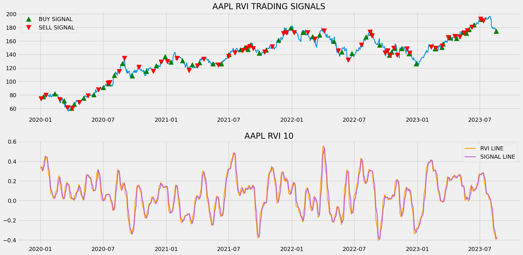
Code Explanation: We are plotting the components of the Relative Vigor Index along with the buy and sell signals generated by the crossover trading strategy. We can observe that whenever the previous reading of the RVI line is below the previous reading of the Signal Line and the current reading of the RVI line is above the current reading of the Signal line, a green-colored buy signal is plotted in the chart. Similarly, whenever the previous reading of the RVI line is above the previous reading of the Signal Line and the current reading of the RVI line is below the current reading of the Signal line, a red-colored sell signal is plotted in the chart.

Step-6: Creating our Position

In this step, we are going to create a list that indicates 1 if we hold the stock or 0 if we don’t own or hold the stock.

Python Implementation:

# STOCK POSITION

position = []
for i in range(len(rvi_signal)):
    if rvi_signal[i] > 1:
        position.append(0)
    else:
        position.append(1)
        
for i in range(len(aapl['close'])):
    if rvi_signal[i] == 1:
        position[i] = 1
    elif rvi_signal[i] == -1:
        position[i] = 0
    else:
        position[i] = position[i-1]
        
close_price = aapl['close']
rvi = aapl['rvi']
signal_line = aapl['signal_line']
rvi_signal = pd.DataFrame(rvi_signal).rename(columns = {0:'rvi_signal'}).set_index(aapl.index)
position = pd.DataFrame(position).rename(columns = {0:'rvi_position'}).set_index(aapl.index)

frames = [close_price, rvi, signal_line, rvi_signal, position]
strategy = pd.concat(frames, join = 'inner', axis = 1)

strategy

Output:

Code Explanation: First, we are creating an empty list named ‘position’. We are passing two for-loops, one is to generate values for the ‘position’ list to just match the length of the ‘signal’ list. The other for-loop is the one we are using to generate actual position values. Inside the second for-loop, we are iterating over the values of the ‘signal’ list, and the values of the ‘position’ list get appended concerning which condition gets satisfied. The value of the position remains 1 if we hold the stock or remains 0 if we sold or don’t own the stock. Finally, we are doing some data manipulations to combine all the created lists into one dataframe.

From the output being shown, we can see that in the first row our position in the stock has remained 1 (since there isn’t any change in the Relative Vigor Index signal) but our position suddenly turned to -1 as we sold the stock when the Relative Vigor Index trading signal represents a sell signal (-1). Our position will remain 0 until some changes in the trading signal occur. Now it’s time to do implement some backtesting process!

Step-7: Backtesting

Before moving on, it is essential to know what backtesting is. Backtesting is the process of seeing how well our trading strategy has performed on the given stock data. In our case, we are going to implement a backtesting process for our Relative Vigor Index trading strategy over the Apple stock data.

Python Implementation:

# BACKTESTING

aapl_ret = pd.DataFrame(np.diff(aapl['close'])).rename(columns = {0:'returns'})
rvi_strategy_ret = []

for i in range(len(aapl_ret)):
    returns = aapl_ret['returns'][i]*strategy['rvi_position'][i]
    rvi_strategy_ret.append(returns)
    
rvi_strategy_ret_df = pd.DataFrame(rvi_strategy_ret).rename(columns = {0:'rvi_returns'})
investment_value = 100000
rvi_investment_ret = []

for i in range(len(rvi_strategy_ret_df['rvi_returns'])):
    number_of_stocks = floor(investment_value/aapl['close'][i])
    returns = number_of_stocks*rvi_strategy_ret_df['rvi_returns'][i]
    rvi_investment_ret.append(returns)

rvi_investment_ret_df = pd.DataFrame(rvi_investment_ret).rename(columns = {0:'investment_returns'})
total_investment_ret = round(sum(rvi_investment_ret_df['investment_returns']), 2)
profit_percentage = floor((total_investment_ret/investment_value)*100)
print(cl('Profit gained from the RVI strategy by investing $100k in AAPL : {}'.format(total_investment_ret), attrs = ['bold']))
print(cl('Profit percentage of the RVI strategy : {}%'.format(profit_percentage), attrs = ['bold']))

Output:

Profit gained from the RVI strategy by investing $100k in AAPL : 58307.54
Profit percentage of the RVI strategy : 58%

Code Explanation: First, we are calculating the returns of the Apple stock using the ‘diff’ function provided by the NumPy package and we have stored it as a dataframe in the ‘aapl_ret’ variable. Next, we are passing a for-loop to iterate over the values of the ‘aapl_ret’ variable to calculate the returns we gained from our RVI trading strategy, and these returns values are appended to the ‘rvi_strategy_ret’ list. Next, we are converting the ‘rvi_strategy_ret’ list into a dataframe and storing it in the ‘rvi_strategy_ret_df’ variable.

Next comes the backtesting process. We are going to backtest our strategy by investing a hundred thousand USD into our trading strategy. So first, we are storing the amount of investment into the ‘investment_value’ variable. After that, we are calculating the number of Apple stocks we can buy using the investment amount. You can notice that I’ve used the ‘floor’ function provided by the Math package because, while dividing the investment amount by the closing price of Apple stock, it spits out an output with decimal numbers. The number of stocks should be an integer but not a decimal number. Using the ‘floor’ function, we can cut out the decimals. Remember that the ‘floor’ function is way more complex than the ‘round’ function. Then, we pass a for-loop to find the investment returns followed by some data manipulation tasks.

Finally, we are printing the total return we got by investing a hundred thousand into our trading strategy and it is revealed that we have made an approximate profit of fifty-eight thousand USD in one year. That’s not bad! Now, let’s compare our returns with SPY ETF (an ETF designed to track the S&P 500 stock market index) returns.

Step-8: SPY ETF Comparison

While this step is optional, it is highly recommended as it enables us to assess the performance of our trading strategy against a benchmark (SPY ETF). Here, we’ll extract SPY ETF data using the ‘get_historical_data’ function and compare the returns from the SPY ETF with the returns generated by our trading strategy applied to Apple stock.

Python Implementation:

# SPY ETF COMPARISON

def get_benchmark(start_date, investment_value):
    spy = get_historical_data('SPY', start_date)['close']
    benchmark = pd.DataFrame(np.diff(spy)).rename(columns = {0:'benchmark_returns'})
    
    investment_value = investment_value
    benchmark_investment_ret = []
    
    for i in range(len(benchmark['benchmark_returns'])):
        number_of_stocks = floor(investment_value/spy[i])
        returns = number_of_stocks*benchmark['benchmark_returns'][i]
        benchmark_investment_ret.append(returns)

    benchmark_investment_ret_df = pd.DataFrame(benchmark_investment_ret).rename(columns = {0:'investment_returns'})
    return benchmark_investment_ret_df

benchmark = get_benchmark('2020-01-01', 100000)
investment_value = 100000
total_benchmark_investment_ret = round(sum(benchmark['investment_returns']), 2)
benchmark_profit_percentage = floor((total_benchmark_investment_ret/investment_value)*100)
print(cl('Benchmark profit by investing $100k : {}'.format(total_benchmark_investment_ret), attrs = ['bold']))
print(cl('Benchmark Profit percentage : {}%'.format(benchmark_profit_percentage), attrs = ['bold']))
print(cl('RVI Strategy profit is {}% higher than the Benchmark Profit'.format(profit_percentage - benchmark_profit_percentage), attrs = ['bold']))

Output:

Benchmark profit by investing $100k : 40181.36
Benchmark Profit percentage : 40%
RVI Strategy profit is 18% higher than the Benchmark Profit

Code Explanation: The code used in this step is almost similar to the one used in the previous backtesting step but, instead of investing in Apple, we are investing in SPY ETF by not implementing any trading strategies. From the output, we can see that our Relative Vigor Index crossover trading strategy has outperformed the SPY ETF by 18%. That’s great!

Final Thoughts!

After an exhaustive process of crushing both theory and coding parts, we have successfully learned what the Relative Vigor Index is all about, the mathematics behind the indicator, and how a simple trading strategy based on it can be implemented in Python.

Even though we managed to surpass the results of the SPY ETF, we are still lagging from those of the actual Apple returns. This may be because the Relative Vigor Index is prone to revealing a lot of false signals when the market is ranging and this can also be observed in the chart represented while discussing the buy and sell signals generated by our crossover trading strategy.

The only way to tackle this problem is to accompany the Relative Vigor Index with another technical indicator that acts as a filter whose only task is to classify the false signals from the authentic ones. Since the Relative Vigor Index is a directional indicator (the indicator’s movement is directly proportional to that of the actual market), choosing a non-directional indicator and especially a volatility type would act as a great filter which ultimately leads us in achieving the desired results from the real-world market.

With that said, you’ve reached the end of the article. If you forgot to follow any of the coding parts, don’t worry. I’ve provided the full source code at the end of the article. Hope you learned something new and useful from this article.

Relative Vigor Index (RVI)

RVI line calculation

Signal line calculation

Implementation in Python

Step-1: Importing Packages

Step-2: Extracting data from EODHD

Step-3: Relative Vigor Index Calculation

Step-4: Creating the trading strategy

Step-5: Plotting the trading signals

Step-6: Creating our Position

Step-7: Backtesting

Step-8: SPY ETF Comparison

Final Thoughts!

Related Articles

Backtesting Technical Analysis Strategies with Excel(SMA, RSI, MACD)

Financial Statement Analysis with Excel

Portfolio Risk Management with Excel

GARCH Analysis on Volatility Patterns

Microsoft Excel Stock Market Dashboard

Real-Time Market Data in Google Sheets with WebSocket