

Time series analysis is a critical component of understanding and predicting trends in various fields such as finance, economics, and environmental science. Two common methods used for smoothing time series data are simple, or equally weighted, Moving Averages (SMA) and Exponentially Weighted Moving Averages (EWMA). In this article, we will delve into the characteristics, advantages, and applications of both approaches.
Additionally, we will demonstrate the practical application of these techniques by deriving volatility estimates from financial time series. We will use the Euro Stoxx 50 market index as an example and highlight the main differences by comparing the two results
Quick jump:
An Introduction to Simple Moving Averages
A moving average is calculated on a rolling estimation sample. In other words, we can set a window of fixed length n, roll it through time and then compute the mean of each sample obtained by adding a new (most recent) observation and taking off the oldest one. This window is often referred to as look-back period. As the name suggests, the same weight is assigned to each observation in the sample. A simple formulation is:

where 

The advantages of this method surely lie in its simplicity and easy interpretability. By equally weighting all data points within its chosen timeframe, SMAs provide a smooth, undisturbed trend line, effectively filtering out the noise inherent in day-to-day market fluctuations and allowing the identification of long-term trends.
Despite being widely used by practitioners, SMAs also come with some pitfalls. One of the main issues is known as the leverage effect, indicating a phenomenon where sudden spikes or outliers in data have a long-lasting impact on the results of moving averages. Let’s consider an exceptionally high return occurring today. If tomorrow we compute the 30-day volatility based on closing prices and include the abnormal return, our volatility forecast will be very high. However, in exactly 30 days (or 22 if we consider only business days), it will suddenly drop to a much lower level on a day when absolutely nothing happened in the markets. This occurrence is simply because the extreme return dropped out of the moving estimation sample. As long as this extreme return stays within the data window, the volatility forecast remains high. We will explore this exact case in the example below.
Exponentially Weighted Moving Averages
Unlike the equal weighting approach, exponentially weighted moving averages (EWMA) add more weight on recent observations. This characteristic makes EWMA particularly useful in capturing short-term volatility dynamics and less prone to the leverage effect issues associated with SMA. By incorporating a smoothing factor 𝜆 that dictates the rate at which past data diminishes in relevance, the model can be tailored to reflect the desired responsiveness to recent market movements. The higher is 𝜆, the more weight would be attributed to past returns when computing the volatility. For constant 

Following this approach, and assuming mean asset returns equal to zero, we can compute EWMA estimates of variances and covariances as follows:


The rightmost part of the last two equations shows a recursive closed-form formulation for variance and covariance in the EWMA case.
An example
Data
For our example, we will use time series data of one of the most known market indices, the Euro Stoxx 50, to compute risk measures for this asset and highlight the main differences obtained by comparing the results of these two techniques. The data sample spans from January 2018 to November 2023, encompassing a total of 1509 observations.
To retrieve our data through the EOD API service, we first need to download and import the EOD Python package, and then authenticate using your personal API key. It’s recommendable to save your API keys in the environment variable.
pip install eodimport os
# load the key from the environment variables
api_key = os.environ['API_EOD']
import eod
client = EodHistoricalData(api_key)1. Use the “demo” API key to test our data from a limited set of tickers without registering: AAPL.US | TSLA.US | VTI.US | AMZN.US | BTC-USD | EUR-USD
Real-Time Data and all of the APIs (except Bulk) are included without API calls limitations with these tickers and the demo key.
2. Register to get your free API key (limited to 20 API calls per day) with access to: End-Of-Day Historical Data with only the past year for any ticker, and the List of tickers per Exchange.
3. To unlock your API key, we recommend to choose the subscription plan which covers your needs.
At this point, we are all set to run our first query. Historical prices can be downloaded using the client.get_prices_eod method by passing the stock ticker, data frequency, sorting criteria, and start data as arguments to the function. The query returns an object structured as list of a dictionaries containing daily price and volume information. For practicality, we apply the pandas function to convert it into a formatted table. Finally, we compute the daily logarithmic returns that will be used to calculate our volatility estimates.
stoxx_data = client.get_prices_eod("STOXX.INDX", period="d", order='a', from_="2018-01-01")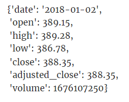
stoxx_ts = pd.DataFrame(stoxx_data).set_index("date")["adjusted_close"]
rets = np.log(stoxx_ts/stoxx_ts.shift(1))[1:]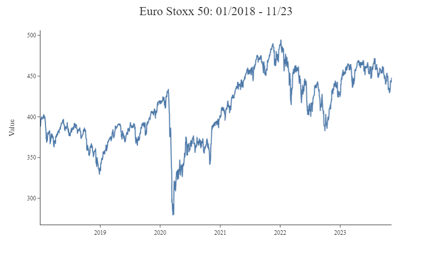
SMA Volatility Estimates
In this example we construct three different equally weighted moving average volatility estimates for the Euro Stoxx 50 index, with T = 30 days, 60 days and 90 days respectively. The pandas rolling function allows us to iterate through the times series keeping a fixed look-back period. As we are dealing with daily returns, volatilities are multiplied by the square root of 250 (business days in a year) to obtain an annualized measure.
std30 = rets.rolling(30).std()*np.sqrt(250)
std60 = rets.rolling(60).std()*np.sqrt(250)
std90 = rets.rolling(90).std()*np.sqrt(250)
std_roll = pd.DataFrame({'30-day vols': std30, '60-day vols': std60, '90-day vols': std90})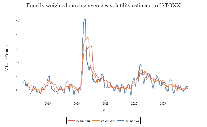
As we can see, the European index reacted quite strongly to the COVID-19 news. The 30-day volatility jumped from ~15% to over 60%! The 60-day and 90-day volatility never exceed the 50%, demonstrating a higher smoothness due to the longer rolling window. It’s interesting to not how the these two, the peak was reached after compared to short-term volatilities, showing a lagging effect, and that all the volatilities have a sudden drop after exactly 30, 60 and 90 days, when nothing special happened in the market.
EWMA Volatility Estimates
The effect of using a different value of lambda in EWMA volatility forecasts can be quite substantial. The graph shows volatility estimates obtained using different lambda values, 𝜆 = (0.90, 0.97, 0.99). Note how, for high levels of 𝜆, the EWMA becomes much less reactive, while persistence improves. This is similar to what was obtained in the SMA case above by increasing the length of the rolling window.
def EWMA_Volatility(rets, lam):
    sq_rets_sp500 = (rets**2).values
    EWMA_var = np.zeros(len(sq_rets_sp500))

    for r in range(1, len(sq_rets_sp500)):
        EWMA_var[r] = (1-lam)*sq_rets_sp500[r] + lam*EWMA_var[r-1]

    EWMA_vol = np.sqrt(EWMA_var*250)
    return pd.Series(EWMA_vol, index=rets.index, name ="EWMA Vol {}".format(lam))[1:]

ewma99_stoxx = EWMA_Volatility(rets, 0.99)
ewma97_stoxx = EWMA_Volatility(rets, 0.97)
ewma90_stoxx = EWMA_Volatility(rets, 0.90)
ewma_all = pd.DataFrame({'𝜆=0.99': ewma99_stoxx,'𝜆=0.97': ewma97_stoxx,'𝜆=0.90': ewma90_stoxx}, index=ewma90_stoxx.index)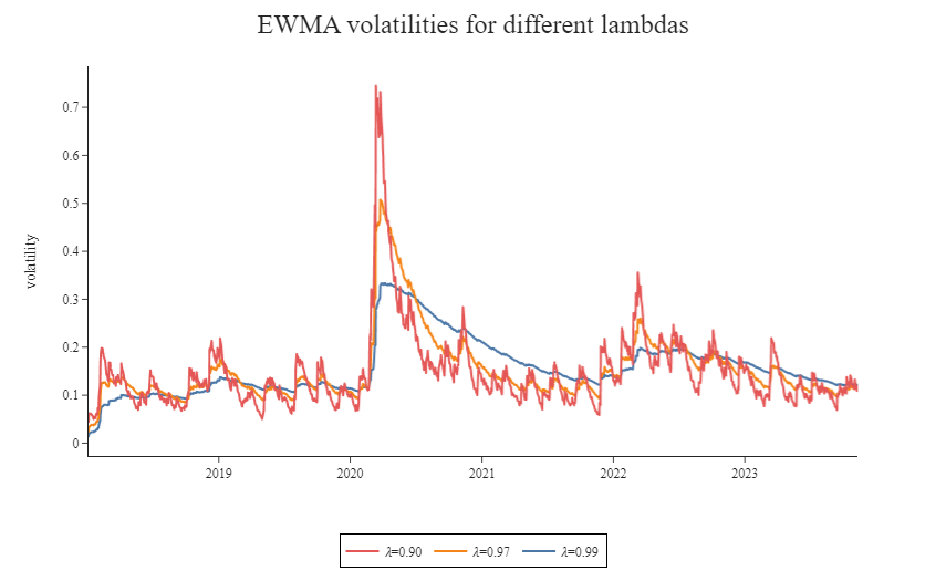
A final comparison
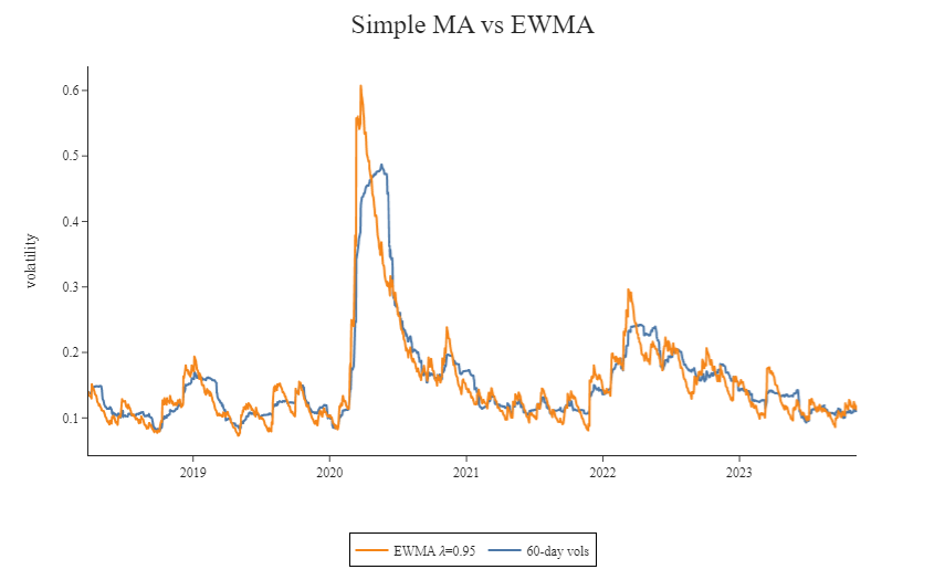
Let’s now compare our estimates obtained using a 60-day SMA and EWMA 𝜆=0.95. When displaying the results on the same graph, it is evident how the two methods produce different risk measures. In particular, the EWMA estimate yields higher volatility than the equally weighted estimate but returns to typical levels faster due to its immunity to the leverage effect.
Finally, note that when computing EWMA estimates for covariances, the same value of lambda should be applied to all the variables to guarantee a semi-definite positive covariance matrix. In practice, different asset classes may react differently to market shocks, and imposing the same smoothing constant to all time series may yield less precise results. This constraint represents one of the main disadvantages of EWMA.
Conclusion
Both Simple and Exponentially Weighted Moving Averages play essential roles in time series analysis. SMAs provide a straightforward yet potentially lagging representation of trends. On the contrary, EWMA’s adaptive nature offers a more responsive volatility estimate, particularly suited for capturing short-term fluctuations. In both cases, the choice of window length and the smoothing constant plays an important role in determining the level of persistence and responsiveness. The decision between the two methods ultimately depends on the specific needs of the analysis and the desired trade-off.
Full code available here
Website: baglinifinance.com