Trading predictions using AI and Python

I’ve tried a number of techniques for predicting stock prices including forecasting tools like Facebook Prophet, statistical approaches like the Seasonal Autoregressive Integrated Moving Average (SARIMA) model, machine learning techniques like Polynomial Regression, and finally an AI recurrent neural network (RNN).

There are a number of AI models and techniques but I’ve found an Long Short-Term Memory (LSTM) model gets the best results. An LSTM model is a type of recurrent neural network (RNN) architecture designed to effectively handle sequence prediction problems. Unlike traditional feedforward neural networks, LSTM has a memory-like architecture that allows it to maintain contextual information over long sequences, making it ideal for time-series prediction, natural language processing, and other sequence-dependent tasks. It overcomes the limitations of basic RNNs by addressing issues like vanishing and exploding gradients, thereby enabling the model to capture long-term dependencies in the data. This makes LSTMs a popular choice for complex tasks that require the understanding of data over extended time periods.

I’ve created a proof of concept to show you how it works.

Register & Get Data

Preparation

• Install Python and PIP, ideally the latest.

• Create yourself a Python project with a file called “main.py“.

• Create a directory within your project called “data“.

• Create yourself a virtual environment within your project and load it.

trading-ai-lstm $ python3 -m venv venv
trading-ai-lstm $ source venv/.bin/activate
(venv) trading-ai-lstm $

• Create yourself a, “requirements.txt” file that looks like this.

pandas
numpy
scikit-learn
scipy
matplotlib
tensorflow
eodhd
python-dotenv

• Make sure you have upgraded PIP within your virtual environment and install the dependencies.

(venv) trading-ai-lstm $ pip install --upgrade pip

(venv) trading-ai-lstm $ python3 -m pip install -r requirements.txt

I have added my EODHD API’s API key into a .env file that looks like this.

API_TOKEN=<YOUR_API_KEY_GOES_HERE>

Register & Get Data

That should be ready now. If you are using VSCode and would like to use the same, “.vscode/settings.json” file as me, here it is.

{
  "python.formatting.provider": "none",
  "python.formatting.blackArgs": ["--line-length", "160"],
  "python.linting.flake8Args": [
    "--max-line-length=160",
    "--ignore=E203,E266,E501,W503,F403,F401,C901"
  ],
  "python.analysis.diagnosticSeverityOverrides": {
    "reportUnusedImport": "information",
    "reportMissingImports": "none"
  },
  "[python]": {
    "editor.defaultFormatter": "ms-python.black-formatter"
  }
}

I’ve create a Github repo for this in case you get stuck.

Building up the code

The first step is you will want to import the necessary libraries.

import os
os.environ["TF_CPP_MIN_LOG_LEVEL"] = "1"

import pickle
import pandas as pd
import numpy as np
from dotenv import load_dotenv
from sklearn.metrics import mean_squared_error, mean_absolute_error
from tensorflow.keras.models import Sequential
from tensorflow.keras.layers import LSTM, Dense, Dropout
from tensorflow.keras.models import load_model
from sklearn.preprocessing import MinMaxScaler
import matplotlib.pyplot as plt
from eodhd import APIClient

TensorFlow produces a lot of warnings and debug information by default. I prefer the output to look nice and tidy so I hide them. That’s what that os.environ line is doing after the “os” import.

When training Machine Learning and AI models, it requires a lot of fine tuning. This is done with something called hyperparameters. This is a really complicated topic and an art on it’s own. The optimal hyperparameters will depend on a number of factors. Based on the daily S&P 500 data I retrieve from EODHD API’s, I’ve started with some fairly common options. Feel free to adjust them to find improve the results. I would leave the sequence length at 20 for now.

# Configurable hyperparameters
seq_length = 20
batch_size = 64
lstm_units = 50
epochs = 100

The next step is I want to retrieve my EODHD API’s API_TOKEN from my .env file.

Register & Get Data

# Load environment variables from the .env file
load_dotenv()

# Retrieve the API key
API_TOKEN = os.getenv("API_TOKEN")

if API_TOKEN is not None:
    print(f"API key loaded: {API_TOKEN[:4]}********")
else:
    raise LookupError("Failed to load API key.")

Nothing too complicated here, just make sure you have a valid EODHD API’s API_TOKEN to be able to retrieve the data.

I’ve created a number of repeatable functions. I’ll explain what they do when we actually use them below. I’ve included comments to explain what is happening within the functions.

def get_ohlc_data(use_cache: bool = False) -> pd.DataFrame:
    ohlcv_file = "data/ohlcv.csv"

    if use_cache:
        if os.path.exists(ohlcv_file):
            return pd.read_csv(ohlcv_file, index_col=None)
        else:
            api = APIClient(API_TOKEN)
            df = api.get_historical_data(
                symbol="HSPX.LSE",
                interval="d",
                iso8601_start="2010-05-17",
                iso8601_end="2023-10-04",
            )
            df.to_csv(ohlcv_file, index=False)
            return df
    else:
        api = APIClient(API_TOKEN)
        return api.get_historical_data(
            symbol="HSPX.LSE",
            interval="d",
            iso8601_start="2010-05-17",
            iso8601_end="2023-10-04",
        )

def create_sequences(data, seq_length):
    x, y = [], []
    for i in range(len(data) - seq_length):
        x.append(data[i : i + seq_length])
        y.append(data[i + seq_length, 3])  # The prediction target "close" is the 4th column (index 3)
    return np.array(x), np.array(y)

def get_features(df: pd.DataFrame = None, feature_columns: list = ["open", "high", "low", "close", "volume"]) -> list:
    return df[feature_columns].values

def get_target(df: pd.DataFrame = None, target_column: str = "close") -> list:
    return df[target_column].values

def get_scaler(use_cache: bool = True) -> MinMaxScaler:
    scaler_file = "data/scaler.pkl"

    if use_cache:
        if os.path.exists(scaler_file):
            # Load the scaler
            with open(scaler_file, "rb") as f:
                return pickle.load(f)
        else:
            scaler = MinMaxScaler(feature_range=(0, 1))
            with open(scaler_file, "wb") as f:
                pickle.dump(scaler, f)
            return scaler
    else:
        return MinMaxScaler(feature_range=(0, 1))

def scale_features(scaler: MinMaxScaler = None, features: list = []):
    return scaler.fit_transform(features)

def get_lstm_model(use_cache: bool = False) -> Sequential:
    model_file = "data/lstm_model.h5"

    if use_cache:
        if os.path.exists(model_file):
            # Load the model
            return load_model(model_file)
        else:
            # Train the LSTM model and save it
            model = Sequential()
            model.add(LSTM(units=lstm_units, activation='tanh', input_shape=(seq_length, 5)))
            model.add(Dropout(0.2))
            model.add(Dense(units=1))

            model.compile(optimizer="adam", loss="mean_squared_error")
            model.fit(x_train, y_train, epochs=epochs, batch_size=batch_size, validation_data=(x_test, y_test))

            # Save the entire model to a HDF5 file
            model.save(model_file)

            return model

    else:
        # Train the LSTM model
        model = Sequential()
        model.add(LSTM(units=lstm_units, activation='tanh', input_shape=(seq_length, 5)))
        model.add(Dropout(0.2))
        model.add(Dense(units=1))

        model.compile(optimizer="adam", loss="mean_squared_error")
        model.fit(x_train, y_train, epochs=epochs, batch_size=batch_size, validation_data=(x_test, y_test))

        return model

def get_predicted_x_test_prices(x_test: np.ndarray = None):
    predicted = model.predict(x_test)

    # Create a zero-filled matrix to aid in inverse transformation
    zero_filled_matrix = np.zeros((predicted.shape[0], 5))

    # Replace the 'close' column of zero_filled_matrix with the predicted values
    zero_filled_matrix[:, 3] = np.squeeze(predicted)

    # Perform inverse transformation
    return scaler.inverse_transform(zero_filled_matrix)[:, 3]

def plot_x_test_actual_vs_predicted(actual_close_prices: list = [], predicted_x_test_close_prices = []) -> None:
    # Plotting the actual and predicted close prices
    plt.figure(figsize=(14, 7))
    plt.plot(actual_close_prices, label="Actual Close Prices", color="blue")
    plt.plot(predicted_x_test_close_prices, label="Predicted Close Prices", color="red")
    plt.title("Actual vs Predicted Close Prices")
    plt.xlabel("Time")
    plt.ylabel("Price")
    plt.legend()
    plt.show()

def predict_next_close(df: pd.DataFrame = None, scaler: MinMaxScaler = None) -> float:
    # Take the last X days of data and scale it
    last_x_days = df.iloc[-seq_length:][["open", "high", "low", "close", "volume"]].values
    last_x_days_scaled = scaler.transform(last_x_days)

    # Reshape this data to be a single sequence and make the prediction
    last_x_days_scaled = np.reshape(last_x_days_scaled, (1, seq_length, 5))

    # Predict the future close price
    future_close_price = model.predict(last_x_days_scaled)

    # Create a zero-filled matrix for the inverse transformation
    zero_filled_matrix = np.zeros((1, 5))

    # Put the predicted value in the 'close' column (index 3)
    zero_filled_matrix[0, 3] = np.squeeze(future_close_price)

    # Perform the inverse transformation to get the future price on the original scale
    return scaler.inverse_transform(zero_filled_matrix)[0, 3]

def evaluate_model(x_test: list = []) -> None:
    # Evaluate the model
    y_pred = model.predict(x_test)
    mse = mean_squared_error(y_test, y_pred)
    mae = mean_absolute_error(y_test, y_pred)
    rmse = np.sqrt(mse)

    print(f"Mean Squared Error: {mse}")
    print(f"Mean Absolute Error: {mae}")
    print(f"Root Mean Squared Error: {rmse}")

There is one point I just want to highlight in the code above. I’ve included a “use_cache” variable in several of the functions. The intention of this is to avoid sending API calls to EODHD API’s repeatedly for no reason, and to avoid re-training the model repeatedly using the same daily data for no reason. If you enable the “use_cache” variable it to save the data to files in the “data/” directory. If the data doesn’t exist it will create it, and if it exists it will load it. If you are running the script repeatedly it’s much more efficient this way. If you would like to generate new data each time just disable the “use_cache” when the function runs or just clear the files in the “data/” directory. It will have the same effect.

Now we dive into the main code…

if __name__ == "__main__":
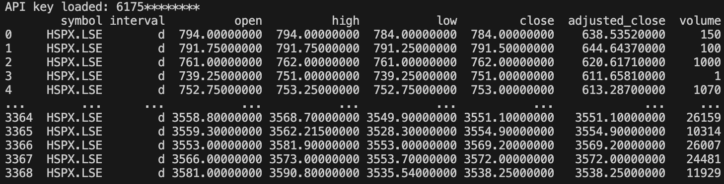
    # Retrieve 3369 days of S&P 500 data
    df = get_ohlc_data(use_cache=True)
    print(df)

We first retrieve our OHLCV data EODHD API’s and store it in a Pandas Dataframe called “df“. OHLCV stands for Open, High, Low, Close, and Volume which are typical fields you would have for trading candle data. You also will notice I have enabled the caching as described above. I also optionally print the data on the screen.

I’ll explain the next code block in one go…

    features = get_features(df)
    target = get_target(df)

    scaler = get_scaler(use_cache=True)
    scaled_features = scale_features(scaler, features)

    x, y = create_sequences(scaled_features, seq_length)

    train_size = int(0.8 * len(x))  # Create a train/test split of 80/20%
    x_train, x_test = x[:train_size], x[train_size:]
    y_train, y_test = y[:train_size], y[train_size:]

    # Re-shape input to fit lstm layer
    x_train = np.reshape(x_train, (x_train.shape[0], seq_length, 5))  # 5 features
    x_test = np.reshape(x_test, (x_test.shape[0], seq_length, 5))  # 5 features

• “features” contains a list of inputs we will use to predict our target I.e. “close“.
• “target” contains a list of the target values I.e. “close“.
• “scaler” is a technique used to normalise numbers to make them comparable. For example we have a close of 784 as our first row, and a close of 3538 on the last row. Just because the last row has a higher value doesn’t mean it’s necessarily more important in terms of a prediction. We want them to be comparable, and this is how it’s done.
• “scaled_features” is the result of the scaling and what we will use to train our AI model.
• “x_train” and “x_test” are our sets will use to train our AI model and then test it. I’ve used an 80/20 split which is fairly common. 80% of our trading data will be used for training the AI model, and 20% of the data will be used to test the model. The “x” means it’s the features, the inputs.
• “y_train” and “y_test” is similar to above but it will just contain the target values I.e. “close“
• Finally, the data needs to be re-shaped to fit into an LSTM layer.

I have created a function to either train the model or load a trained model.

model = get_lstm_model(use_cache=True)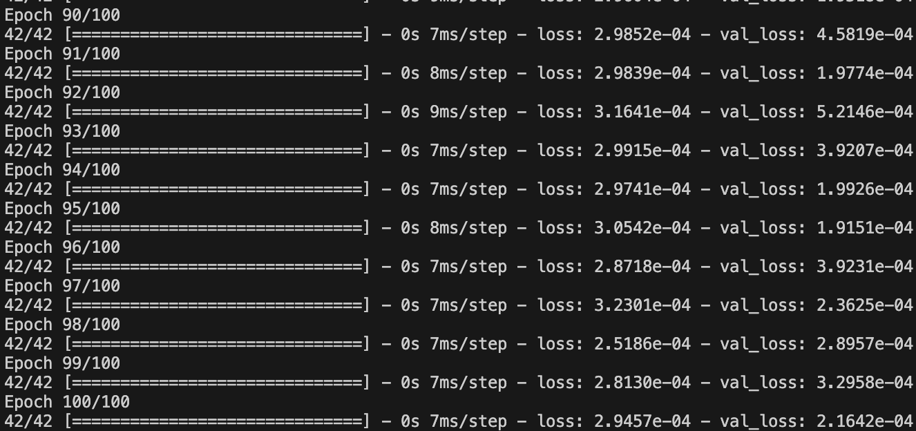

The screenshot above shows a snippet of the training process. You will notice that as the training starts the “loss” and “val_loss” won’t be very close as as the training progresses you should the numbers getting closer together.

• loss: This is the mean squared error (MSE) computed on the training dataset. It reflects the “cost” or “error” between predicted and true labels for each training epoch. The aim is to minimize this value over epochs.
• val_loss: This is the mean squared error computed on the validation dataset. The validation dataset is a subset of the data that the model has never seen during training. It’s an indicator of how well the model generalises to unseen data.

If you want to see a list of the predicted close prices on the test set, you can use this code.

    predicted_x_test_close_prices = get_predicted_x_test_prices(x_test)
    print("Predicted close prices:", predicted_x_test_close_prices)

It’s not all that helpful or easy to visualise on it’s own. If we plot the actual closing prices against the predicted closing prices (remember 20% of the full dataset), it looks like this.

    # Plot the actual and predicted close prices for the test data
    plot_x_test_actual_vs_predicted(df["close"].tail(len(predicted_x_test_close_prices)).values, predicted_x_test_close_prices)

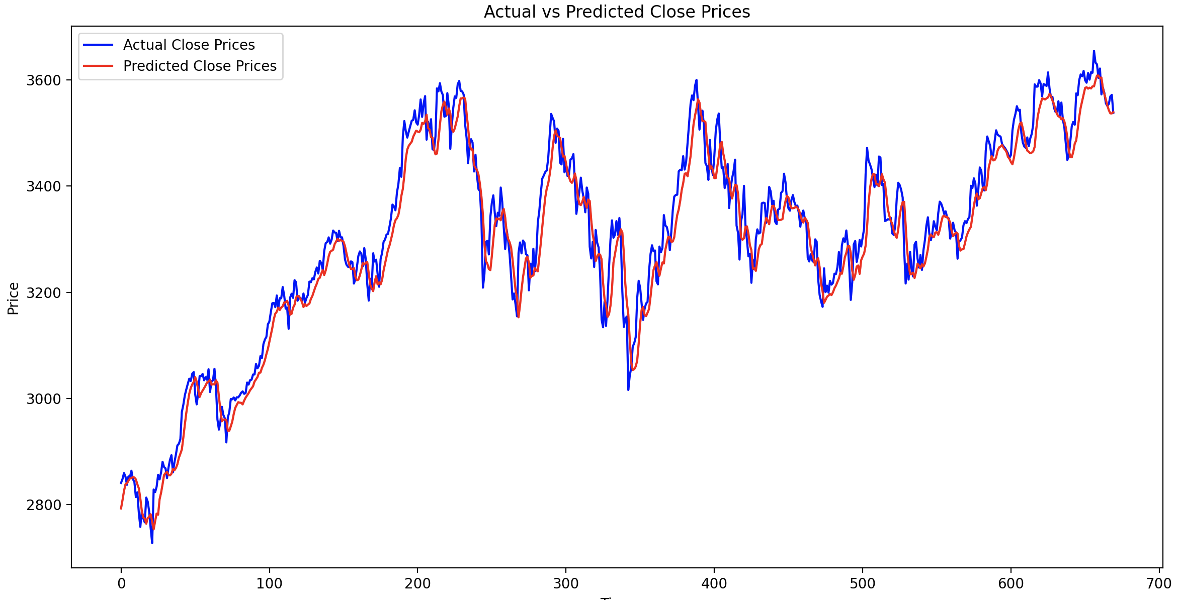
You can see it’s done a pretty good job a predicting the closing price using the testing phase.

Now the part you are probably waiting for. Can we find out what the predicted closing price is tomorrow?

   # Predict the next close price
    predicted_next_close =  predict_next_close(df, scaler)
    print("Predicted next close price:", predicted_next_close)

Predicted next close price: 3536.906685638428

This is just a basic example for academic purposes, and just the start. Following on from this you can look at adding more training data, experimenting with the hyperparameters, or training models on different markets and intervals.

If you want to evaluate the model you can include this.

    # Evaluate the model
    evaluate_model(x_test)

Which in my case is…

Mean Squared Error: 0.00021641664334765608
Mean Absolute Error: 0.01157513692221611
Root Mean Squared Error: 0.014711106122506767

The mean_squared_error and mean_absolute_error functions from scikit-learn’s metrics module are used to calculate MSE and MAE, respectively. The Root Mean Squared Error (RMSE) is calculated as the square root of MSE.

These metrics provide a quantitative evaluation of the model’s performance, while the plot helps in visually assessing how closely the predicted values match with the actual values.

Register & Get Data